QGIS Automation: One Task, 4 Methods, Timed on 2 Cities
Published
You can automate a repetitive QGIS workflow four ways: Batch Processing for one tool across many files, the Graphical Modeler for a chain of tools you will re-run, a PyQGIS script for loops and exact control, or an AI agent inside QGIS when you want the result from one plain-English message.
 workflow four ways: Batch Processing for one tool across many files, the Graphical Modeler for a chain of tools you will re-run, a
The tutorials I read teach one of those four in isolation on a toy example, and none tests what happens when you run the workflow a second time on a new city. On 7 November 2026, I took one multi-step task (built-up area per district from 180,602 OpenStreetMap buildings in Bielefeld, Germany), ran it through all four methods in QGIS 3.44.15, and then re-ran all four on Münster (135,577 buildings, 6 districts). Every method passed on both cities, though one Graphical Modeler run first finished "OK" while writing 1,058 polygons instead of 10.
8.1s
PyQGIS script on Bielefeld (7.4 s on Münster)
62.7s
Graphical Modeler in QGIS (44.5 s headless)
60s
AI Agent re-run on Münster from 1 sentence
1,058rows
Written instead of 10 on a silent model bug
What is QGIS automation?
QGIS automation means running a processing tool or a chain of tools across layers without clicking through each dialog by hand. Underneath every method sits the QGIS Processing framework, the same engine that powers the Processing Toolbox. Because the tools are identical whether you call them from a batch table, a Graphical Modeler diagram, a Python script, or the qgis_process command-line tool, choosing an automation method is really choosing how you want to wire those tools together and what file you want left on disk for next month.
The task and the data we tested on
I picked a job that comes up all the time in urban planning and consultancy: for each city district, clip the buildings to the district boundary, count the footprints, sum their area in square metres, buffer the clipped buildings by 25 m and dissolve them into a single built-up polygon, and save one clean GeoPackage with one row per district.
If a building crosses a district border, it is clipped and counted once in each district it touches. Both cities use OpenStreetMap data from BBBike PBF extracts (ODbL, OpenStreetMap contributors), reprojected to EPSG:25832 (ETRS89 / UTM zone 32N) for all measurements.
- City 1, Bielefeld: 180,602 building polygons across 10 districts (
admin_level=9), producing 115,002 clipped building pieces. Two raw OSM buildings had invalid geometries and were repaired once with Fix geometries so all four methods started from the same clean files. - City 2, Münster (the re-run): 135,577 building polygons across 6 districts, producing 116,382 clipped pieces.
Before running any of the four methods, I wrote an independent reference in plain PyQGIS geometry calls (QgsSpatialIndex, geometry.intersection(), unaryUnion(), and buffer(25, 5), without calling Processing algorithms) and saved a checker script. A method passed only if it produced one GeoPackage with a built_up polygon layer in EPSG:25832, exact building counts per district, footprint area within 0.5% of the reference, built-up hectares within 1%, and no hand editing afterwards.
Method 1: Batch Processing
Every tool in the Processing Toolbox has a Run as Batch Process button in the bottom-left corner of its dialog. It turns the dialog into a spreadsheet where each row is one run of that single tool.
For our task, batch processing handles the per-district Clip and the per-district Buffer cleanly, because those two steps repeat the exact same algorithm across the 10 districts. It cannot do the whole workflow in one go, though, because Batch Processing only runs one tool at a time and leaves you with 10 separate output layers that you still have to merge and join back together.
Reproject and split the inputs
Run Reproject layer (Vector general) on the buildings to EPSG:25832. Then run Split vector layer (Vector general) on the districts layer using the name field, which writes one GeoPackage per district into a folder.
Run Clip as a batch across all districts
Open Clip (Vector overlay), click Run as Batch Process, and add one row per district file. Set the reprojected buildings as the Input layer, use Autofill to populate the district overlays and output table names (clip_<district>), and untick Load layers on completion. On Bielefeld, all 10 rows finished in 13.7 s (1.0 to 4.2 s per district).
Run Buffer as a batch with Dissolve switched on
Open Buffer (Vector geometry) in batch mode: one row per clipped layer, Distance 25, Segments 5, and Dissolve result ticked. The 10 Bielefeld buffers ran in 27.7 s.
Merge, aggregate, and join the table back together
Run Merge vector layers twice (once on the 10 clip layers, once on the 10 buffer layers). Run Aggregate (Vector geometry) on the merged clips grouped by the layer field to get building_count (count($id)) and building_area_m2 (sum(area($geometry))). Run Refactor fields (Vector table) on the merged buffers to compute built_up_ha with the $area / 10000 field calculator expression, then Join attributes by field value (Vector general) on district to produce the single output layer.
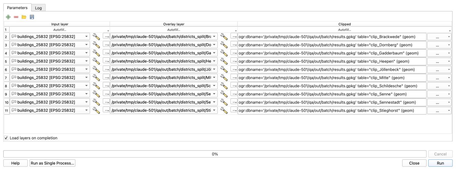
Across the 9 runs (8 different algorithms), total tool execution time on Bielefeld was 62.0 seconds, and every district count matched the reference. On Münster, the tool time dropped to 39.8 seconds for 6 districts, but I had to rebuild the 6-row batch tables and re-run all 9 steps by hand. When your workflow is a chain of different tools rather than one tool repeated across 50 files, Batch Processing is the wrong shape.
Method 2: The Graphical Modeler
The Graphical Modeler (Processing > Graphical Modeler) lets you wire a chain of Processing tools into a single diagram and save it as a .model3 file. Once built, the model appears in your Processing Toolbox like any native tool.
You might expect to need a loop over the districts inside the Modeler, but you don't. By running Intersection between the buildings and districts first, every building piece inherits its district's name attribute, so Aggregate and Dissolve grouped by name produce one row per district in a single pass. (You could also use a spatial join if you didn't need buildings split strictly at the district line.)
Add the three model inputs
In a new model, add two Vector Layer inputs (Polygons) named Buildings and Districts, and one Number input named Buffer distance (m) with a default value of 25.
Reproject both inputs and intersect them
Add two Reproject layer nodes targeting EPSG:25832. Connect both to an Intersection node (Buildings as Input, Districts as Overlay). In Intersection's Input fields to keep, limit the building fields to osm_id only, and in Overlay fields to keep, keep name.
Branch into Aggregate for counts and Dissolve + Buffer for geometry
From Intersection, connect one branch to Aggregate grouped by name to compute count($id) and sum(area($geometry)). Connect a second branch from Intersection to Dissolve (field name) followed by Buffer (linked to your Buffer distance (m) input, 5 segments).
Join the branches and format the output table
Add Join attributes by field value to attach the Aggregate table to the buffered polygons on name, then Refactor fields to rename name to district and compute built_up_ha as $area / 10000. Mark the output as built_up and save the model as built_up_by_district.model3.
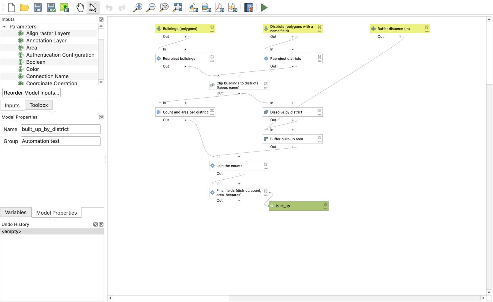
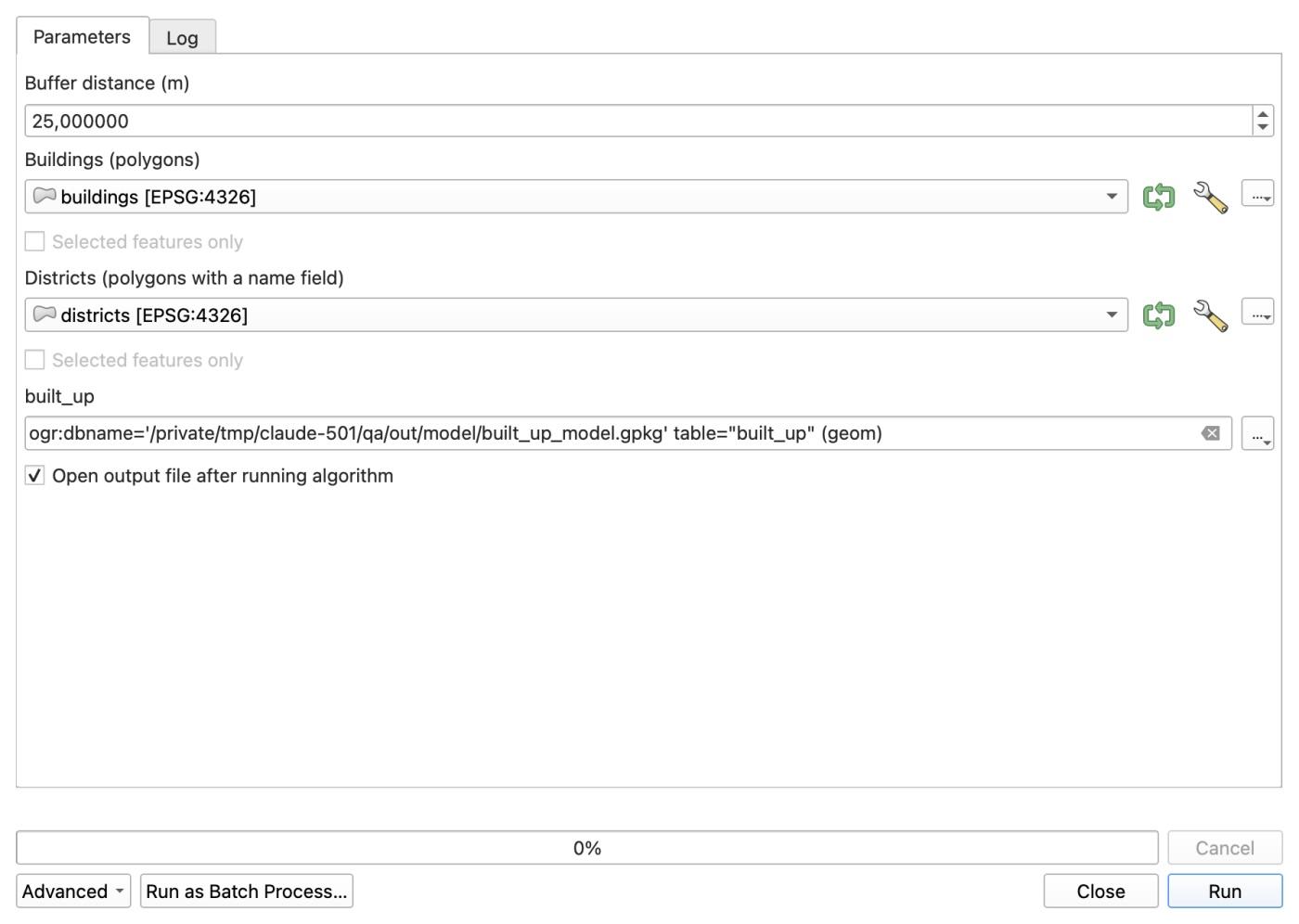
Running the model from its dialog on Bielefeld took 62.7 seconds and passed every check. Better still, the exact same .model3 file ran from the macOS terminal without opening a QGIS window via qgis_process in 44.5 seconds.
The real payoff showed up on the Münster re-run. I opened the same model dialog, selected muenster_buildings and muenster_districts in the two drop-downs, and clicked Run. It finished in 67.2 seconds with zero edits to the model.
Method 3: A PyQGIS script in the Python Console
If you are comfortable with Python, a script inside Plugins > Python Console > Show Editor gives you a real for loop, the inputs as variables at the top of the file, and no merge steps.
Here is the 38-line script (built_up_by_district.py) I ran in QGIS 3.44.15, with the file paths shortened:
# Built-up area by district. Run in the QGIS Python console (Plugins > Python Console > Show Editor > Run).
# Change the first five lines for a new city.
BUILDINGS = "data/bielefeld_buildings.gpkg"
DISTRICTS = "data/bielefeld_districts.gpkg"
NAME_FIELD = "name"
BUFFER_M = 25
OUT = "out/script/built_up_script.gpkg"

import processing
from qgis.core import (QgsVectorLayer, QgsCoordinateReferenceSystem, QgsFeature, QgsField, QgsFields, QgsGeometry)
from qgis.PyQt.QtCore import QVariant

crs = QgsCoordinateReferenceSystem("EPSG:25832")   # metric, Germany
def run(alg, **p):
    return processing.run(alg, p)["OUTPUT"]

buildings = run("native:reprojectlayer", INPUT=BUILDINGS, TARGET_CRS=crs, OUTPUT="memory:")
districts = run("native:reprojectlayer", INPUT=DISTRICTS, TARGET_CRS=crs, OUTPUT="memory:")

result = QgsVectorLayer("MultiPolygon?crs=EPSG:25832", "built_up", "memory")
result.dataProvider().addAttributes([QgsField("district", QVariant.String), QgsField("building_count", QVariant.Int),
                                     QgsField("building_area_m2", QVariant.Double), QgsField("built_up_ha", QVariant.Double)])
result.updateFields()

for d in districts.getFeatures():
    one = run("native:extractbyexpression", INPUT=districts, EXPRESSION=f"$id = {d.id()}", OUTPUT="memory:")
    clipped = run("native:clip", INPUT=buildings, OVERLAY=one, OUTPUT="memory:")
    area = sum(f.geometry().area() for f in clipped.getFeatures())
    built_up = run("native:buffer", INPUT=clipped, DISTANCE=BUFFER_M, SEGMENTS=5, DISSOLVE=True, OUTPUT="memory:")
    geom = next(built_up.getFeatures()).geometry()
    f = QgsFeature(result.fields())
    f.setGeometry(geom)
    f.setAttributes([d[NAME_FIELD], clipped.featureCount(), area, geom.area() / 10000])
    result.dataProvider().addFeature(f)
    print(d[NAME_FIELD], clipped.featureCount(), round(area), round(geom.area() / 10000, 1))

processing.run("native:savefeatures", {"INPUT": result, "OUTPUT": OUT, "LAYER_NAME": "built_up"})
print("saved", OUT)
The script keeps every intermediate layer in memory and loops over the districts, and it was by far the fastest method (we did not profile why). It finished Bielefeld in 8.1 seconds and matched the independent reference to 0.00% on every district.
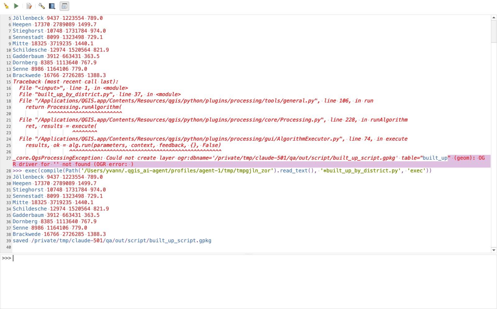
To re-run it on Münster, I changed three lines at the top (BUILDINGS, DISTRICTS, and OUT) and clicked the green Run Script play button. It finished in 7.4 seconds. If you want to learn how processing.run works in detail, see our PyQGIS guide.
How the four methods compared on both cities
Here is what we measured across all four methods on 7 November 2026:
| Batch Processing | Graphical Modeler | PyQGIS script | AI Agent (Medium, Balanced) | |
|---|---|---|---|---|
| Setup / structure | 9 runs across 8 algorithms (2 batch tables of 10 rows) | 3 inputs + 8 algorithm nodes + 1 output | 38 lines of Python, 5 algorithms | 1 plain-English message (27 tool calls by the agent) |
| Bielefeld run time (10 districts) | 62.0 s of tool time (started one by one) | 62.7 s in dialog (44.5 s via qgis_process) | 8.1 s (after fixing 1 failed save call) | 110 s from Send to the answer table |
| Münster re-run (6 districts) | 39.8 s of tool time (rebuild batch rows and all 9 runs) | 67.2 s (pick 2 new layers, click Run) | 7.4 s (change 3 file path lines, click Run) | 60 s (1 follow-up message of 46 words, 15 tool calls) |
Largest gap vs reference (built_up_ha) | +0.08% | +0.08% | 0.00% | +0.21% |
| What you keep afterwards | ~20 intermediate layers | One .model3 file (runs in UI or headless) | One .py script file | The chat history and your prompt text |
Every method matched the reference building counts and building footprint areas (building_area_m2) to 0.00%. The +0.08% difference on built_up_ha for Batch Processing and the Graphical Modeler comes from $area in Refactor fields measuring on the project ellipsoid, whereas the script and reference used planar geometry().area() in EPSG:25832.
What broke along the way (including a silent wrong answer)
Tutorials rarely show the runs that fail, so I logged every error during the day. The scariest failure was not a crash or a red error banner: it was a Graphical Modeler run that reported success and gave the wrong output.
When I first ran the model headless before limiting the fields on the Intersection node, the log printed:
Model processed OK. Executed 8 algorithm(s) total in 84.548 s.
No error, no warning. When I checked the output GeoPackage, built_up had 1,058 polygons instead of 10.
Here is why: OpenStreetMap buildings have their own name column (the name of a shop, school, or church), and the districts layer also has a name column. When Intersection combined all fields from both layers, the buildings' name stayed name and the district's name was silently renamed to name_2. Downstream, Aggregate and Dissolve grouped by name, so they grouped by building names instead of districts! Limiting Intersection's Input fields to keep to osm_id prevented the collision and dropped the output back to the 10 districts.
Three other things broke and are worth knowing before you automate your own data:
- Invalid OSM geometries stop Processing by default. Two of the 180,602 Bielefeld buildings had self-intersecting rings. Under QGIS's default setting, Clip stops immediately with
Feature (18818404) from 'b' has invalid geometry. Run Fix geometries as your first step whenever your input comes from raw OpenStreetMap. savefeaturesin PyQGIS dislikes GDAL connection strings. On my first script run (10.0 s), passingogr:dbname='...' table="built_up"tonative:savefeaturesraisedOGR driver for '' not found. Pass the plain.gpkgpath inOUTPUTand setLAYER_NAME: "built_up"as a separate parameter.- Loading many intermediate layers crashed our session. QGIS crashed (
SIGSEGV) three times as Processing outputs loaded into the layer tree with Load layers on completion ticked. Unticking it for intermediate batch rows stopped the crashes.
Method 4: Asking an AI agent inside QGIS
We build AI Agent, so this section is about our own plugin. It docks a chat panel inside QGIS, inspects the layers and fields already in your project, calls QGIS Processing tools and PyQGIS itself, and checks the output before answering.
For a one-off job or a two-city project, building an 8-node Graphical Model or debugging a 38-line script is often more setup than the task deserves. I opened a project containing the Bielefeld buildings and districts layers, set the panel to Medium effort and Balanced permissions, and sent one message:
The project has two layers: "buildings" (OSM buildings of Bielefeld, Germany) and "districts" (its 10 city districts, the district name is in the field "name"). For each district: clip the buildings to the district, count the buildings, sum their footprint area in square meters, and build a 25 m buffer around the clipped buildings, dissolved into one built-up polygon, with its area in hectares. Measure in a metric CRS (EPSG:25832). Write one GeoPackage at [output folder]/built_up_agent.gpkg with a single polygon layer named built_up, one feature per district, fields district, building_count, building_area_m2, built_up_ha, in EPSG:25832. Then show me the result table.
(Output paths shortened in both prompts. Transparency note: on the very first attempt, QGIS crashed 9 seconds after I clicked Send with a Qt slot segfault before any answer returned. I re-opened the project, sent the exact same prompt once, and did not re-send after that.)
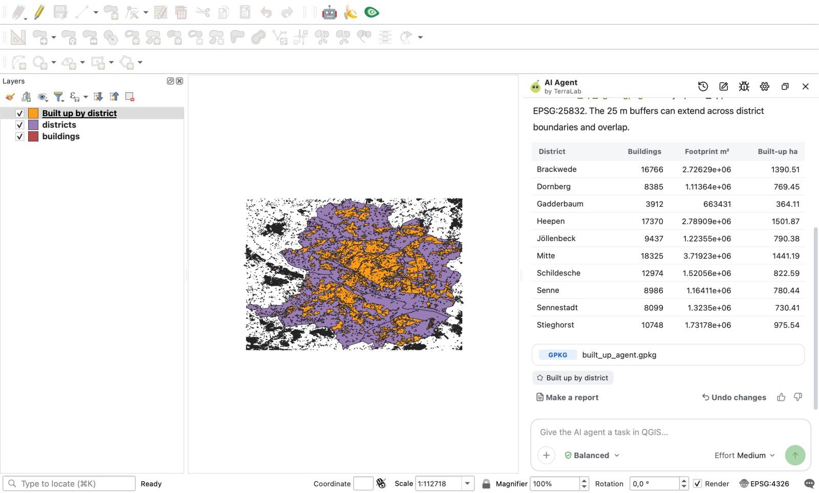
In 110 seconds, the agent ran 27 tool calls (12 run_processing, 7 get_algorithm_help, 4 execute_code, 2 get_layer_info, 1 export_layer, 1 get_features), recovered from one internal Processing error on its own without showing a permission card, wrote the GeoPackage, and printed the 10-district table in the chat. Without being prompted, it also noted in its answer: "The 25 m buffers can extend across district boundaries and overlap."
Then I dragged muenster_buildings and muenster_districts into the project and typed a 46-word follow-up in the same chat:
Now do the same for Münster. I added two layers: "muenster_buildings" and "muenster_districts" (6 districts, the name is in the field "name"). Same fields and same 25 m buffer, in a new GeoPackage at [output folder]/built_up_agent_muenster.gpkg with the layer named built_up. Then show me the result table.
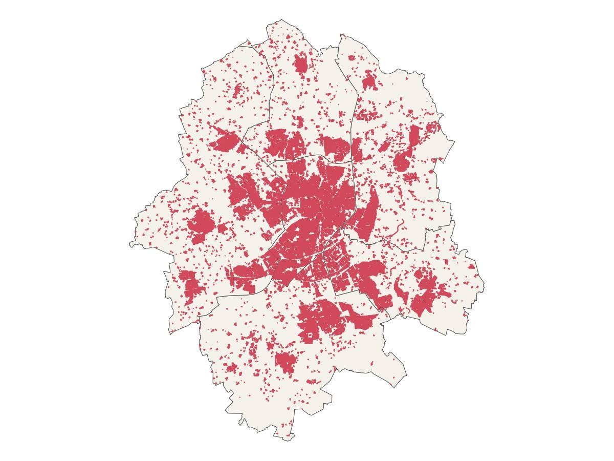
With the first run in the same chat, the agent finished Münster in 60 seconds using 15 tool calls (11 run_processing, 1 export_layer, 1 get_features, 1 zoom_to_layer, 1 execute_code) with zero errors.
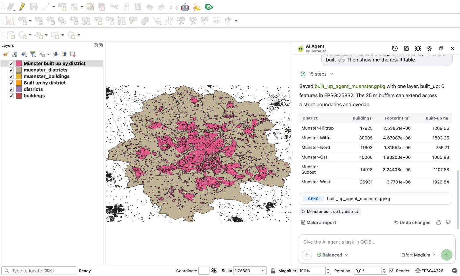
Every building count and footprint area matched the reference to 0.00% on both cities.
Where are the limits? First, the agent's built_up_ha values sat 0.07% to 0.21% above the planar reference (for example, Brackwede came out at 1,390.51 ha vs 1,388.31 ha in the reference; we did not measure which internal step caused that small difference). Second, the exported GeoPackage kept an extra _export_fid column. Third, and most important for automation: the agent plans its steps fresh on every message (27 tool calls on Bielefeld, 15 on Münster) and runs inside an open QGIS session, so it does not leave you a .model3 or .py file that you can schedule unattended with cron.
Which QGIS automation method should you pick?
Instead of treating one tool as the winner, match the method to how often you will repeat the job:
- You are running the exact same single tool across 10 to 100 files: use Batch Processing. It is built into every Processing dialog, costs nothing, and needs zero code. Stop using it as soon as your workflow chains three or four different tools together.
- You or your team will run a multi-step chain every month, or on a server schedule: build it in the Graphical Modeler. You get a single
.model3file you can share with colleagues who don't write Python, and you can execute it headless from a shell script or scheduled task viaqgis_process. - You need custom loops, exact planar control, or the fastest execution speed: write a PyQGIS script. Our 38-line script ran 8 to 9 times faster than the Modeler on both cities.
- You have a complex task to run once, twice, or across a few project variations today: use an AI agent inside QGIS like AI Agent (or see our broader overview on the QGIS AI hub). You skip hunting for exact tool names and re-run on a second city with one sentence. The Free plan gives 5 tasks a month at Low effort; these tests ran at Medium, which comes with Pro (49 EUR / month excl. VAT, 300 tasks).
How we measured this. All tests ran on 7 November 2026 on one Apple Silicon Mac (macOS 27.0.1, arm64) in an isolated QGIS 3.44.15-Solothurn session (Python 3.12.11) with AI Agent 1.9.4 (Medium effort, Balanced mode). Machine load varied during the day, so compare the timings as orders of magnitude, not as CPU benchmarks. We measured machine wall-clock execution time and step counts, not the human minutes a GIS analyst takes to click together a model or write a script from scratch. All inputs, the .model3 file, the .py scripts, the reference checker, and the raw JSON logs are stored in our experiment archive.
Frequently asked questions
How do I automate a repetitive workflow in QGIS?
You have four main options depending on how often the job repeats. For a single tool across many files, click Run as Batch Process inside the tool's dialog. For a multi-step chain you will re-run regularly, wire the tools together in Processing > Graphical Modeler and save a .model3 file. For loops and fastest performance, write a Python script using processing.run() in the QGIS Python Console. For one-off or few-time analyses where you don't want to wire nodes or write code, describe the workflow in plain words in an agent plugin such as AI Agent.
Should I use the QGIS Graphical Modeler or Python (PyQGIS)?
Use the Graphical Modeler when your workflow is a straight chain of Processing algorithms and you want a visual .model3 file that non-programmers on your team can open, or that you can run from the command line with qgis_process. Use PyQGIS when you need to loop over features, keep intermediate layers in memory (the script ran in 8.1 s vs 62.7 s for the model in our Bielefeld test), handle errors in code, or control output schemas explicitly.
Can I export a QGIS Graphical Model to a Python script?
Yes. The Graphical Modeler can export a model as a Python Processing script (Export as Script Algorithm), which you can then edit to add loops, variables or custom logic. We did not test the export in this comparison.
Can QGIS run automated workflows on a schedule without opening the app?
Yes. QGIS ships with a command-line utility called qgis_process. You can pass it any native algorithm or any saved .model3 file (for example, qgis_process run model3 --BUILDINGS=... --DISTRICTS=... --built_up=...) from a bash script, Windows Task Scheduler, or cron job without launching the graphical QGIS interface. In our Bielefeld test, the model ran headless through qgis_process in 44.5 seconds.
Read nextWhat Is PyQGIS? A First Script and a Chatbot Code Test
Do it in QGIS by asking for it
AI Agent carries out the task you describe, in your own QGIS project. Free, no card.