Convert Raster to Vector in QGIS: 5 Methods
Published Updated
To convert a raster to vector polygons in QGIS, open Raster > Conversion > Polygonize (Raster to Vector), pick your band, name the output field, and run it. You get one polygon per connected group of pixels sharing a value, with that value in the attribute table. It is the right answer for a classified raster and the wrong one for a photograph. Four other methods cover the rasters polygonize cannot read.
 , open
 Method 2 is a plugin we build, so weigh that section accordingly. It gets the same five lines as the other four.
The short answer
Open the raster's properties and read two things: the band type and the number of distinct values. They pick the method for you.
| Your input | Method | What it costs |
|---|---|---|
| Classified raster (land cover, a slope reclass, a mask) | Method 1, Raster > Conversion > Polygonize | Free, in core QGIS |
| Orthophoto, drone or satellite imagery | Method 2, a segmentation model | Free plugins need an NVIDIA card. Cloud plugins have free tiers, then a subscription |
| Continuous raster (NDVI, slope, a reflectance band) | Method 3, Reclassify by table, then polygonize | Free, in core QGIS |
| DEM or any elevation surface | Method 4, Raster > Extraction > Contour, or Contour Polygons | Free, in core QGIS |
| Scanned paper map or a plan | Method 5, GRASS r.thin plus r.to.vect | Free, and slow. Paid AI tracing exists |
Every menu path, algorithm id and default below was checked against the QGIS 3.44 documentation and the GDAL stable docs on 23 August 2026. Menu paths assume the default QGIS layout, which a plugin can change.
Method 1: Polygonize
Work in a projected CRS. Two steps below take a distance or an area in layer units, and in degrees those numbers mean nothing.
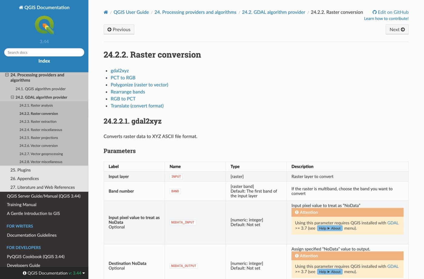
The algorithm is Polygonize (raster to vector), id gdal:polygonize, wrapping the GDAL utility gdal_polygonize.
Open the tool
Raster > Conversion > Polygonize (Raster to Vector), or the Processing Toolbox under GDAL, Raster conversion.
Pick the band
Band 1 unless your classes live elsewhere. One band only, so reduce an RGB raster to a single class band.
Name the field
DN is the default. Rename it, landcover_code rather than DN.
Decide on 8-connectedness
Off by default, so pixels must share a full border to join. Turn it on and diagonally touching pixels join too. Left off, a thin diagonal feature splits into a chain of polygons. On our WorldCover test below it cut the polygon count by 21% and the vertex count by nothing: it groups pixels, it does not smooth them.
Save to a real file
The default is a temporary layer. 100 km2 of 10 m land cover gave us 9,221 polygons and a 4.9 MB GeoPackage, so write straight to a file.
![The QGIS Polygonize dialog: Land cover 10 m [EPSG:32631], Band 1 (Palette), field landcover_code, 8-connectedness unticked, output to a GeoPackage.](/_next/image?url=%2Fblog%2Fraster-to-vector-qgis%2F02_polygonize_dialog.jpg&w=3840&q=75&dpl=dpl_4mcJgn5aTuBLsC5D4Lc9L46y53Pr)
Two things save you time. First, set a NoData value on the class you do not want: GDAL then reads the band's validity mask and skips those pixels instead of wrapping one enormous background polygon around everything. That is the most common complaint about polygonize output, and it is a raster property, not a tool setting.
Second, watch the band type. gdal:polygonize always writes an integer field, so it casts a float band on the way in, and that fails in two ways depending on how the raster stores its values. Neither warns you. A Float32 band goes through Method 3 first.
The staircase and the speckle: sieve first, simplify as a coverage
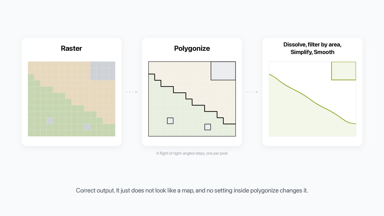
Polygonize traces pixel boundaries, so a diagonal field edge comes back as right-angled steps, one per pixel. A 10 m Sentinel classification gives 10 m stairs.
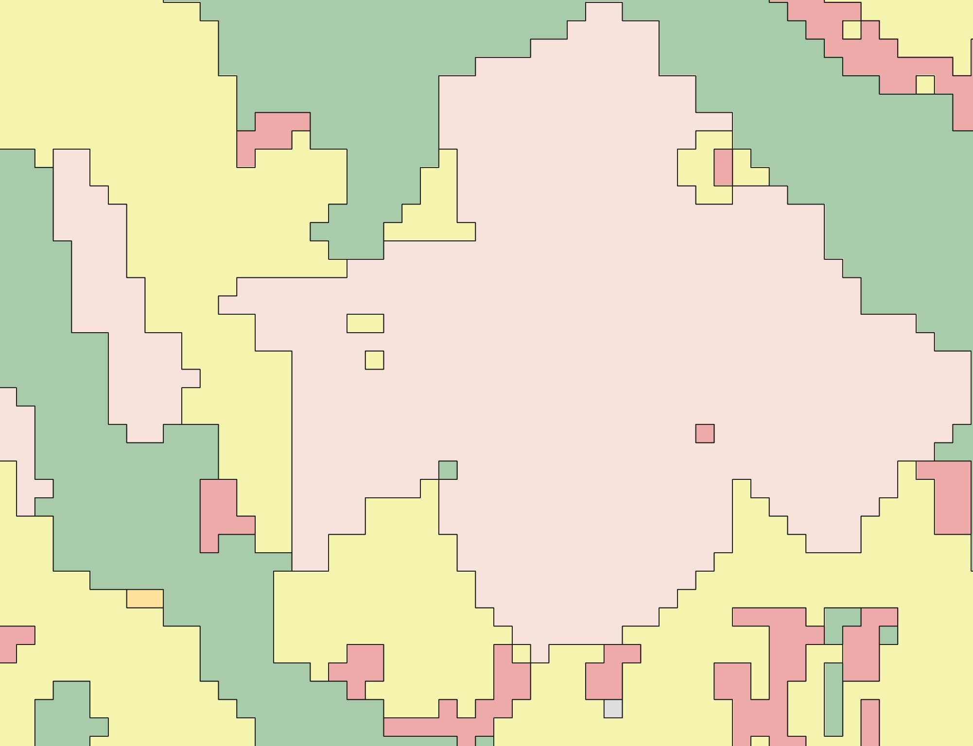
That is correct output, and no setting inside polygonize changes it. What fixes it is one raster step before polygonize and one coverage step after. On a 10 km square of ESA WorldCover around Crest, in the Drôme, polygonize returned 9,221 polygons and 200,656 vertices, and 57% of those polygons were smaller than five pixels. Sieving the raster at 10 pixels first cut that to 2,660 polygons and changed the class of 1.75% of the pixels.
The usual vector fix then breaks the map. QGIS's Simplify works one polygon at a time, so two neighbours simplify their shared edge differently: at a 10 m tolerance that opened 88 ha of gaps and 81 ha of overlaps across the 10,000 ha square. Simplify coverage treats the layer as one mesh and left none.
| Step on the 10 km square | Polygons | Vertices | GeoPackage | Pixels whose class changed | Gaps and overlaps |
|---|---|---|---|---|---|
| Polygonize, default 4-connected | 9,221 | 200,656 | 4.9 MB | 0% | 0 |
| Polygonize, 8-connected | 7,284 | 200,656 | 4.7 MB | 0% | 0 |
| Sieve 5 px, then polygonize | 3,886 | 168,060 | 3.6 MB | 0.94% | 0 |
| Sieve 10 px (the default), then polygonize | 2,660 | 155,920 | 3.2 MB | 1.75% | 0 |
| Sieve 50 px, then polygonize | 1,001 | 122,440 | 2.4 MB | 5.36% | 0 |
| Sieve 10 px, then Simplify at 10 m | 2,660 | 57,896 | 1.5 MB | 4.11% | 169 ha |
| Sieve 10 px, then Simplify coverage at 10 m | 2,660 | 84,984 | 1.9 MB | 2.63% | 0 |
Sieve beats the $area filter for the same reason. Deleting every polygon under 500 m2 removes 5,263 specks, the ones a 5 pixel sieve absorbs, but leaves 94 ha of holes; the sieve hands those pixels to their largest neighbour, so the map stays wall to wall. Of the 51 QGIS YouTube tutorials in our research corpus that name Polygonize, none runs Sieve before it.
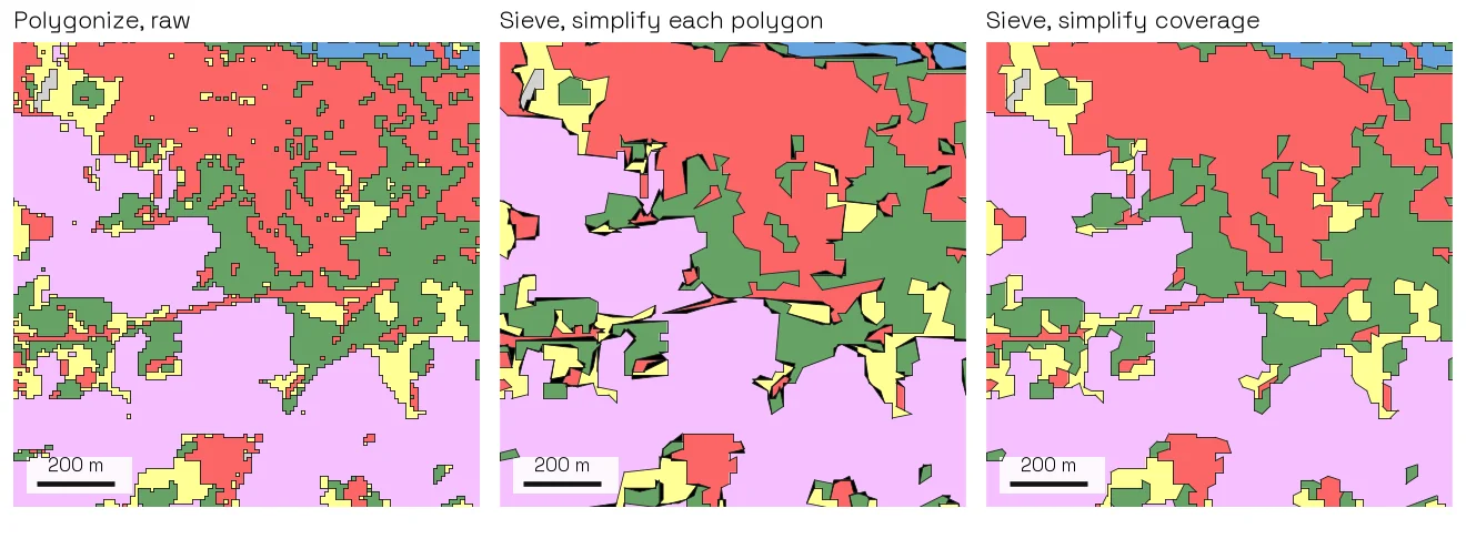
In QGIS, the whole cleanup is four steps, in this order.
Sieve the raster
Raster > Analysis > Sieve, id gdal:sieve, before polygonize. Threshold is in pixels and defaults to 10, which is 1,000 m2 on a 10 m raster. Every patch smaller than that takes the value of its largest neighbour. The class change grows with the threshold: 1.75% of pixels at 10, 8.19% at 100.
Polygonize the sieved raster
Method 1 as above. No Dissolve needed: polygonize already writes one polygon per patch.
Simplify coverage
Processing Toolbox, Vector coverage, native:coveragesimplify, in QGIS since 3.36. Tolerance is in layer units and defaults to 1. On a 10 m raster it removed nothing at 5 m and 45% of the vertices at 10 m, so start at one pixel. Keep plain Simplify for isolated patches that share no edge, such as one class over NoData.
Smooth, but only on curves
native:smoothgeometry, on genuinely curved things: streams, coastlines, vegetation patches. Offset defaults to 0.25, iterations control how round it gets. Set Maximum node angle to smooth to 90 and sharper corners stay sharp, which saves the corners of buildings and parcels.
How we measured this. ESA WorldCover 2021 v200, tile N42E003, a 10 km square centred on Crest (44.728 N, 5.022 E), reprojected to EPSG:32631 at 10 m by nearest neighbour, on 23 September 2026. "Pixels whose class changed" burns the polygons back onto the same grid and compares them with the original raster. Gaps and overlaps are the area no polygon covers and the area two polygons cover. The polygonize, sieve, Simplify and Simplify coverage rows were re-run with the tools shipped in QGIS 3.44.7 (GDAL 3.12, GEOS 3.14) and gave the same counts. One window, one land cover product and one pixel size: a 30 m or 1 m raster moves every number.
Use it when: the raster holds classes as integers.
Skip it when: the band is a float, a photograph or elevation.
Method 2: A segmentation model for photographs
A segmentation model has learned what the objects look like, so it finds them in a photograph where no pixel value separates them. We build one of these, AI Segmentation. This section is about our own tool.
Point polygonize at the same orthophoto and you get noise. A red roof and a red car have similar pixel values, and so do a grey roof and a grey road. The classes exist in your head, not in the file.
Install from the plugin manager
No GPU, no Python environment, no model weights to fetch.
Create an account
It needs one. Free allowance, then €39 a month excluding VAT.
Pick a mode
Both cloud modes send imagery to a server. The small local model stays on your machine.
Run it over your extent
Back comes a polygon layer in the project CRS, with label, class, score, area_m2 and perimeter_m on every feature.
Filter the output
Raw model output needs filtering the way polygonize output needs cleaning. On one run over central Paris I kept 82 polygons out of 635, and those 82 held 84 percent of the built area.
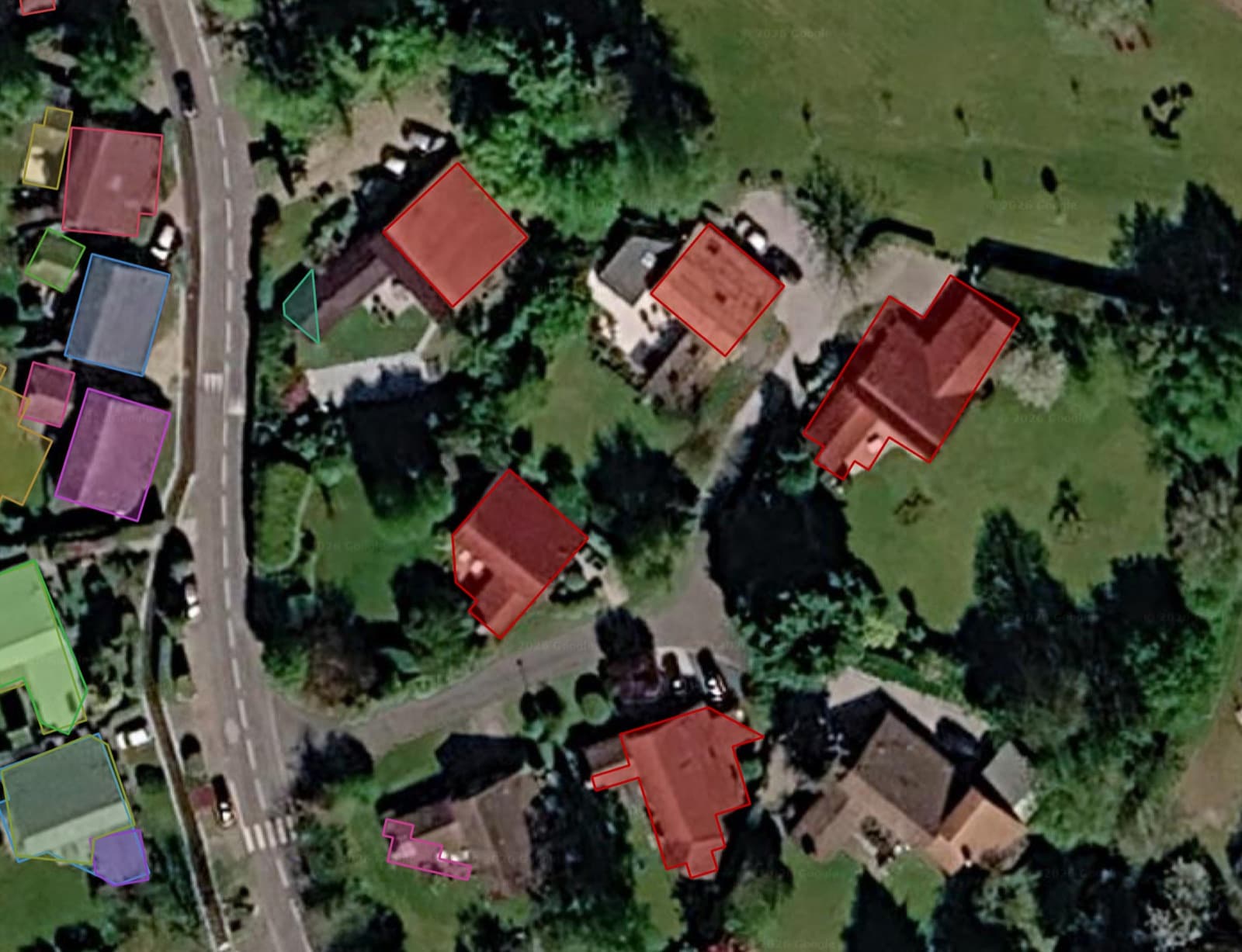
Five other plugins do this job, ours in the last row. Costs and free tiers read 23 August 2026.
| Tool | What you install | GPU | Account | Imagery leaves your machine | What comes out | Cost |
|---|---|---|---|---|---|---|
| Deepness (source) | Plugin manager, then its Python packages and an ONNX model | Optional, CPU works | No | No | Polygon layer, bounding boxes, or a raster | Free |
| Geo-SAM | Plugin manager, then dependencies and model weights from its settings dialog | Optional, clicking runs on CPU | No | No | Polygon layer, pixel-level or simplified | Free |
| samgeo | A Python package in your environment, no QGIS panel | Recommended | No | No | GeoJSON, Shapefile or GeoPackage you load yourself | Free |
| Mapflow (site) | Plugin manager | No | Yes | Yes in the cloud service, your GeoTIFF upload or the tile service you point at. An enterprise on-premise option is offered | Polygon layer | Credits, paid |
| Bunting Labs AI Vectorizer | Plugin manager | No | Yes | Yes, in raster chunks | Vertices into the layer you are digitizing | Trial, then 29 dollars a month |
| AI Segmentation (ours) | Plugin manager | No | Yes | Yes in both cloud modes, no for the small local model | Polygon layer in the project CRS, with label, class, score, area_m2 and perimeter_m | Free allowance, then €39 a month excluding VAT |
One limit each.
- Deepness runs the model you hand it, so you find or train one first.
- Geo-SAM takes clicks and boxes, one object at a time.
- samgeo has no QGIS interface. You write Python.
- Mapflow offers ready-made models for buildings, forest, roads and construction sites.
- Bunting Labs AI Vectorizer follows line work as you digitize.
- AI Segmentation, ours, sends imagery to a server in both cloud modes. Only the small local model stays local.
Use it when: the input is a photograph and there are more objects than you would draw by hand.
Skip it when: the imagery cannot leave your machine, which a local plugin such as Deepness or Geo-SAM can handle.
Try it free in QGIS, no card needed
Method 3: Reclassify, then polygonize
Polygonize on a continuous raster fails in one of two ways, depending on how the values are stored.
Stored as scaled whole numbers, which is how NDVI products ship, you get a polygon for nearly every pixel. I measured 39,801 polygons out of 40,000 pixels on a Sentinel-2 scene.
Stored as raw floats between -1 and 1, the cast to integer flattens every value to -1, 0 or 1 before the trace starts. The same scene came back as 238 polygons in two classes. That looks clean, but the values are gone.
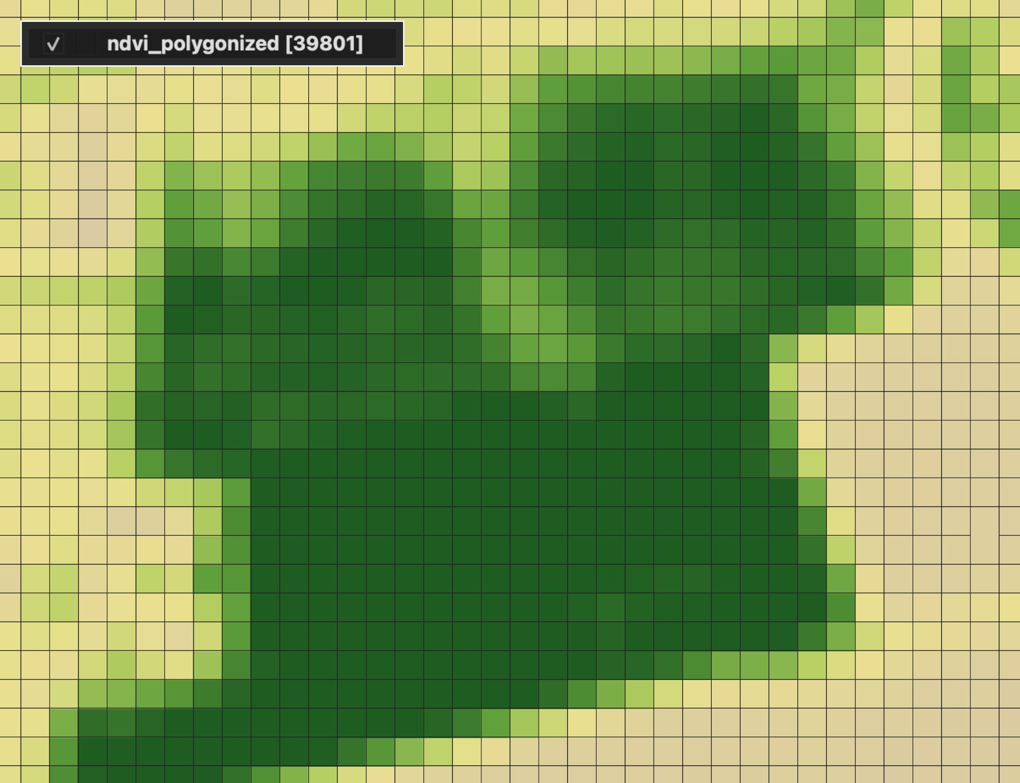
Slope, elevation, temperature and a raw reflectance band all do the same. The tool traces boundaries between integer values, and a continuous raster has none worth tracing. So make the classes yourself, with Reclassify by table, id native:reclassifybytable.
Open Reclassify by table
Processing Toolbox, Raster analysis. The continuous raster is the input.
Type the class table
Three columns: minimum, maximum, new value. It accepts -inf, inf and nan for NoData. A vegetation mask is three rows.
| Minimum | Maximum | Value |
|---|---|---|
| -inf | 0.2 | 1 |
| 0.2 | 0.5 | 2 |
| 0.5 | inf | 3 |
Set the output data type
In the advanced parameters, Output data type defaults to Float32. Set it to Byte or Int16 and polygonize behaves.
Check the range boundaries
Range boundaries defaults to min < value <= max, which decides where a pixel at exactly 0.2 lands. Pick what your class definition means.
Polygonize the result
Run Method 1 on the reclassified raster, then the four cleanup steps.
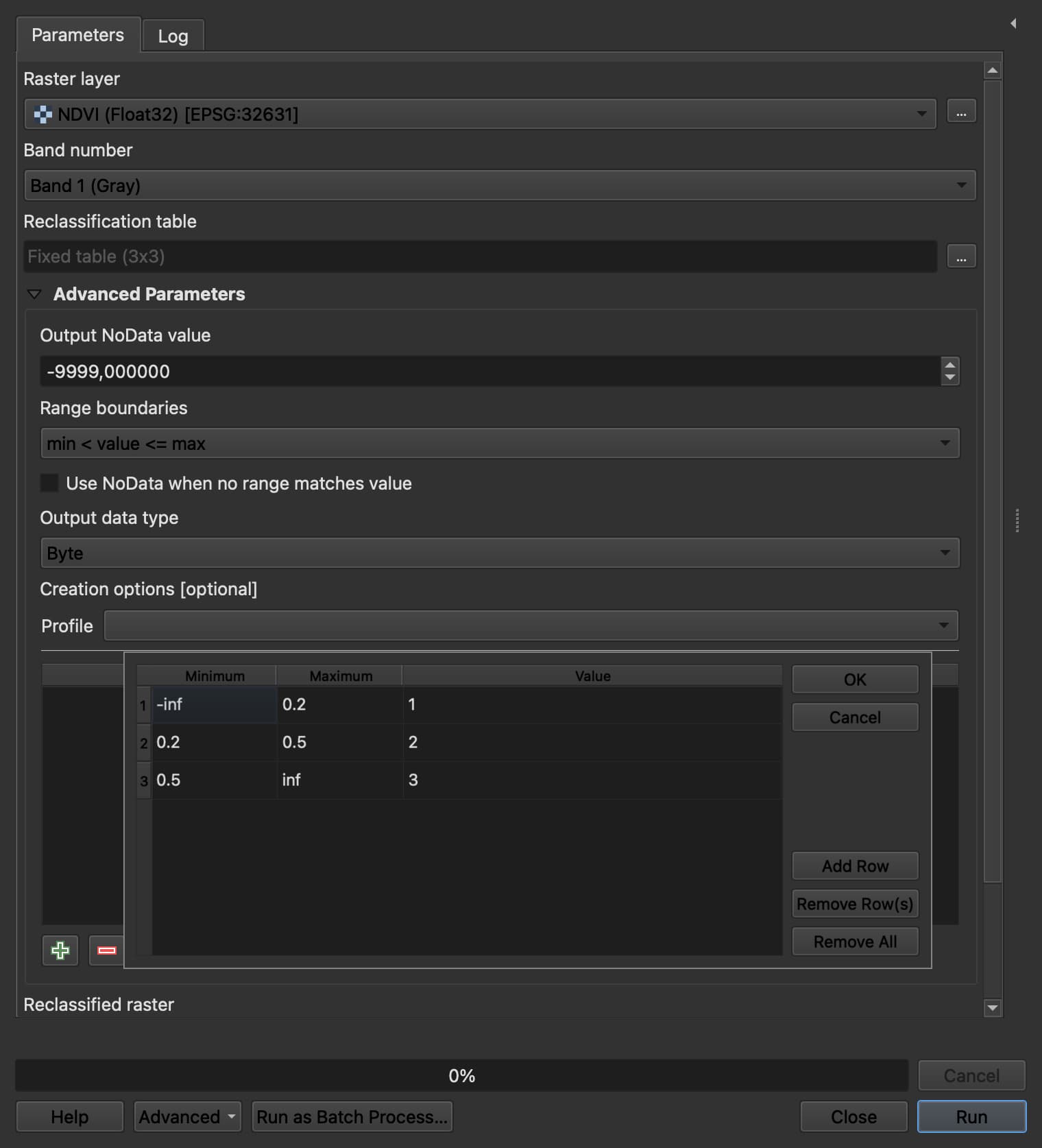
Use it when: you can say in numbers where one class stops and the next starts.
Skip it when: the thing you want is an object rather than a value range.
Method 4: Contours from a DEM
For elevation, do not polygonize. Use Contour at Raster > Extraction > Contour, id gdal:contour.
Open Contour
Raster > Extraction > Contour, with the DEM as input.
Set the interval
Defaults to 10.0 in raster units, so a metric DEM gets a line every 10 m.
Name the attribute
Elevation goes into ELEV by default. Keep it, and label from it.
Decide on Produce 3D vector
Tick it for the height on every vertex. Leave it off for a printed map, since a lot of software drops the Z.
Switch to contour polygons for filled bands
The sibling algorithm gdal:contour_polygon gives filled bands between two elevations, with ELEV_MIN and ELEV_MAX on each polygon. That is the one for a hypsometric map or an inundation extent, and it saves polygonizing a reclassified DEM by hand.

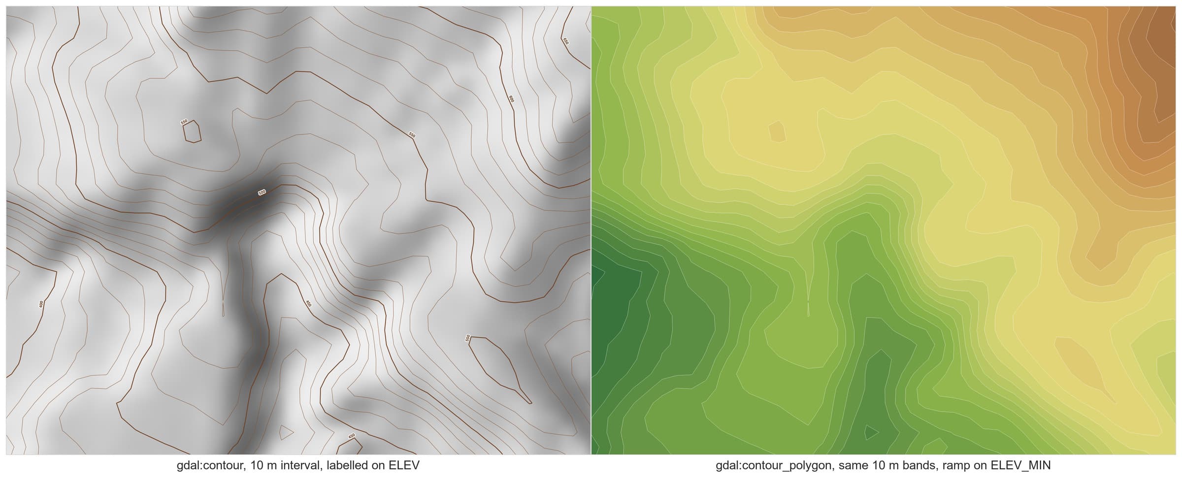
Contours from a lidar DEM come out noisy, because the surface is noisy. Smooth the raster before the contour step, never the lines afterwards: smoothed lines cross each other.
Use it when: the thing you want is a level: elevation, depth, rainfall, concentration.
Skip it when: the raster already holds classes.
Method 5: Scanned paper maps
If you came from ArcGIS looking for the QGIS equivalent of ArcScan, there is not one. Interactive raster tracing, where you click a line on a scan and the tool follows it, is a real gap in QGIS, and I would rather say so than have you hunt the menus. For what else changes when you move over, see QGIS vs ArcGIS Pro.
The free path runs through GRASS, which ships with most QGIS installers.
Threshold the scan
Turn the scanned sheet into a binary raster: line work in one value, paper in the other.
Thin the lines
r.thin reduces each stroke to a single pixel wide.
Vectorize
r.to.vect with feature type line. The GRASS documentation warns that this creates excessive nodes at junctions and dangling spurs, so budget for cleanup.
Two other routes exist. Potrace and AutoTrace run outside QGIS: bitmap in, vector out, then you georeference the result. They are good on high-contrast scans and blind to geography.
Inside QGIS, Bunting Labs AI Vectorizer (QGIS repository listing) autocompletes a line as you digitize, aimed at geologic maps, as-builts and plans. It sends raster chunks to their servers, there is no free tier beyond a trial, and published prices start at 29 dollars a month, read 23 August 2026.
For a handful of features, hand-digitizing with snapping still wins. I would not build a tracing workflow for fewer than about fifty features.
Use it when: the scan carries clean line work and hundreds of features.
Skip it when: the sheet is faint, hatched or annotated over the lines.
What to remember
| What the properties say | Method |
|---|---|
| Integer band, under a hundred distinct values | Method 1, sieve, polygonize, then Simplify coverage |
| Three bands of a photograph | Method 2, a segmentation model |
| Float band, thousands of distinct values | Method 3, reclassify by table, then Method 1 |
| Elevation in metres, or any smooth surface | Method 4, contour or contour polygons |
| A scanned sheet with no class values at all | Method 5, GRASS, or digitize by hand |
The distinct-value count settles it. Under a hundred, somebody has already classified the raster, and polygonize traces those classes cleanly.
In the thousands, nobody has classified anything, so you draw the thresholds yourself in Method 3 or hand the job to a model in Method 2.
The staircase is correct output, and no setting inside polygonize removes it. Sieve the raster first, then Simplify coverage, not Simplify, so neighbours keep one shared edge.
Every cleanup step moves vertices, so compute any area that feeds a report from the raster rather than from the polygons.
Polygonize cannot read a photograph at any setting, because the classes are in your head and not in the file.
Questions people ask
Is raster to polygon the same as raster to vector?
Not quite. Raster to vector covers polygons, lines and points. Raster to polygon is the polygonize route in particular, Raster > Conversion > Polygonize, which is Method 1. The contours in Method 4 are also raster to vector, and they come out as lines.
Why does polygonize give me one giant polygon around everything?
The background class has no NoData value set, so GDAL traces it as real data. Set NoData on that class in the raster's properties, then run Method 1 again.
Why did polygonize create a polygon for almost every pixel?
The raster is continuous, not classified, so almost no two neighbouring pixels hold the same value. Reclassify it first: Method 3.
How do I get rid of the staircase edges?
Sieve the raster before polygonize, then run Simplify coverage at about one pixel, then Smooth on curved features only. Plain Simplify works polygon by polygon and opens gaps between neighbours. Compute areas from the raster if they feed a report.
Does QGIS have an ArcScan equivalent?
No. Core QGIS has no interactive raster tracing. Method 5 has the free path, GRASS r.thin then r.to.vect, and the paid one, the Bunting Labs plugin from 29 dollars a month.
Can I polygonize an aerial photo or a satellite image?
No, and the output will look like static, since a red roof and a red car share pixel values. Use a segmentation model: Method 2.
How do I remove the tiny polygons polygonize creates?
Run Raster > Analysis > Sieve on the raster before polygonize. It merges every patch under the threshold into its largest neighbour. Deleting small polygons afterwards leaves holes instead.
Is raster to vector free in QGIS?
Yes for Methods 1, 3 and 4: polygonize, reclassify, contour and the cleanup algorithms are all core QGIS. Only the photograph case and paid scan tracing cost money.
The building footprints guide walks the filtering step end to end, and the SAM in QGIS post covers which objects these models find well. The QGIS AI hub compares the plugins side by side. If all you need is buildings, our free building footprints tool pulls them from open data in the browser, with no plugin.