How to Georeference a Map or Image in QGIS
Published
To georeference a map or image in QGIS, open Layer > Georeferencer, load the scan with Open Raster, click at least four points you can identify and type their real coordinates, choose Polynomial 1 and a projected target CRS in Transformation Settings, then press Start Georeferencing. QGIS writes a GeoTIFF and adds it to your project.
 , open
 Placing the points is the easy part. The part most tutorials skip is judging the result, because the number QGIS shows you can be zero on a map that is hundreds of metres off. I georeferenced a 1947 USGS map of San Francisco and measured every result against points the fit never saw. The numbers below come from that test.
The short answer
| Your input | Method | Time or cost |
|---|---|---|
| A scan with coordinates printed on it (graticule, grid ticks, corner values) | Method 1, type the printed values | Free. 8 points, then a 34 s warp on a 6,888 x 8,933 px scan |
| A scan with no coordinates, or a photo of a map | Method 1, From Map Canvas on a basemap | Free. Plan on 10 or more points |
| A GeoPDF from USGS or another agency | Open it directly, it is already placed | Free, zero points |
| A quick visual overlay, no accuracy needed | Method 2, the Freehand raster georeferencer plugin | Free plugin |
| Points already read, and you want the fit checked for you | Method 3, an AI agent | 1 message, 99 s in my test |
Before you start
You need QGIS 3.26 or later, where the Georeferencer sits in the Layer menu. I used QGIS 3.44.7. Older tutorials send you to Raster > Georeferencer, which is where it lived before, as the GDAL Georeferencer plugin.
Read the map's collar before you click anything. It tells you three things you will type later: the coordinate system of the printed values, the datum, and the scale. My sample is the USGS San Francisco North, CA quadrangle from 1947, at 1:24,000, which anyone can download from topoView. Its collar says "Polyconic projection. 1927 North American datum", and its corners carry latitudes and longitudes every 7'30". USGS historical maps are public domain.
To make the test honest, I took USGS's own GeoTIFF of that sheet and stripped its georeferencing, so what I loaded into QGIS was a plain 9.2 MB JPEG of 6,888 x 8,933 pixels. That is about 300 dpi, or 2.03 m of ground per pixel. USGS's georeferencing stayed on the side as the answer key.
Where the web gets this wrong
"The lower the RMSE, the better the result." Not with a thin plate spline. That transform bends the image until it passes exactly through every point, so its residuals are always zero. I typed one latitude wrong on purpose, 37°47' instead of 37°47'30", and ran both transforms on the same eight points. Polynomial 1 showed an RMSE of 297 m and put 762 m of it on the bad point. Thin plate spline showed 0.00 m, and the map was up to 594 m off at points it had not been given.
"Enter the coordinates in WGS 84." The printed values on older US maps are often NAD27, and the collar says so. In San Francisco, the same latitude and longitude in NAD27 and in WGS 84 are 93 m apart, 92 m of it east to west. Type them as EPSG:4326 and the whole sheet lands a block away, with residuals that look perfect, because every point moved together. In the Enter Map Coordinates dialog, set the CRS of the points to what the collar says: EPSG:4267 for NAD27.
"Leave the target CRS in degrees." You can, but a flat affine fit in latitude and longitude does not match how a projected map was drawn. With the same eight points, Polynomial 1 gave 2.98 m of RMSE with EPSG:4267 as the target, and 0.72 m with NAD27 / UTM zone 10N (EPSG:26710). Pick a projected CRS on the map's datum, and the fit reads in metres too.
Method 1: The QGIS Georeferencer
This is the built-in tool and the one to learn first. It works for scans with printed coordinates and for scans without them.
Open the scan
Layer > Georeferencer, then File > Open Raster and pick the image. JPEG, PNG and TIFF all work.
Add a control point
Click Add GCP Point, zoom in and click a spot you can identify exactly: a corner of the map frame, a graticule cross, a grid tick. The Enter Map Coordinates dialog opens. Type the printed coordinate. It accepts degrees, minutes and seconds with spaces (-122 25 0), decimal degrees, or projected metres. Set the CRS under the fields to the one the collar names.
Or take the coordinate from the map canvas
When the scan has no coordinates, load a basemap in the main QGIS window first (the basemap guide has the clicks), then press From Map Canvas and click the same spot on it. QGIS fills in the coordinates and the CRS for you.
Spread the points
Put one near each corner and a few in the middle. Points bunched in one area fit that area and let the rest of the sheet drift. I used the four corners of the map frame and the four graticule crosses inside it.
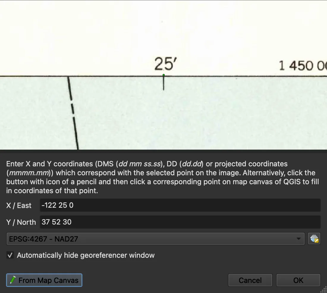
Every point you add goes into a .points file next to the image. Keep it: the Georeferencer loads it on its own the next time you open the same scan, and you can fix a point instead of starting over.
Choose the transformation
Settings > Transformation Settings holds the choice that matters most. The QGIS 3.44 manual lists seven transforms, with these minimum point counts:
| Transformation | Minimum points | Use it for |
|---|---|---|
| Linear | 2 | A clean scan that only needs a shift and a scale. Writes a world file, no warp |
| Helmert | 2 | The same plus a rotation |
| Polynomial 1 | 3 | Most flat scans of printed maps. Straight lines stay straight |
| Projective | 4 | A photo of a map taken at an angle |
| Polynomial 2 | 6 | A curled or bent sheet. Distorts the edges past your points |
| Polynomial 3 | 10 | Same, stronger. Rarely worth it |
| Thin plate spline | 10 according to the manual | Damaged or hand-drawn maps with many points. Hides errors, see above |
My rule: start with Polynomial 1. Move to anything more flexible only when its residuals show a pattern, such as every point on one side pulling the same way, and never because a higher number looked worse.
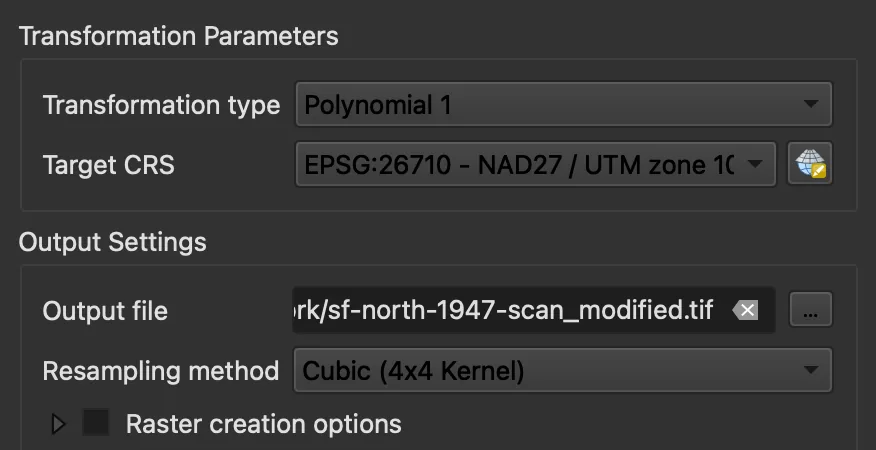
Two settings on that dialog save trouble later. Resampling method changes how the warped pixels look: nearest neighbour keeps the original colours, cubic reads better on a scan. And the output has no compression by default: my 9.2 MB JPEG became a 187 MB GeoTIFF. Open Raster creation options and pick a compression profile if the file will travel.
Read the residuals
Once you have more points than the transform needs, QGIS shows each point's residual in the GCP table and a mean error in the status bar, both in pixels for a scan without coordinates.
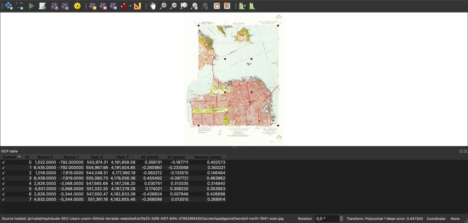
To judge a pixel figure, turn it into metres and compare it with what the map itself can deliver.
- Metres per pixel. Multiply the scale denominator by the size of a scanned pixel. At 300 dpi one pixel is 0.0847 mm, so on a 1:24,000 map it covers 2.03 m. My 0.447 pixels is 0.9 m.
- What the map can promise. US National Map Accuracy Standards require 90 percent of well-defined points on a 1:24,000 sheet to be within 1/50 inch, which USGS gives as 12.2 m. A stricter rule of thumb is the width of a drawn line, 0.2 mm on the sheet, which is 4.8 m at 1:24,000.
- Points the fit never saw. A residual only says the points agree with each other. I kept the eight graticule ticks along the edges out of the fit and measured where the result put them: 1.0 m off on average, 1.6 m at worst.
So the georeferencing added about a metre of error to a map that only promises 12 m. On an old sheet, the map is almost always the limit, not your clicks.
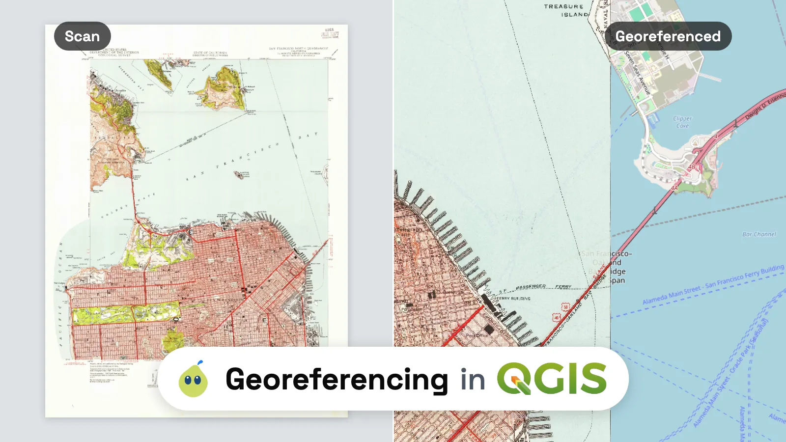
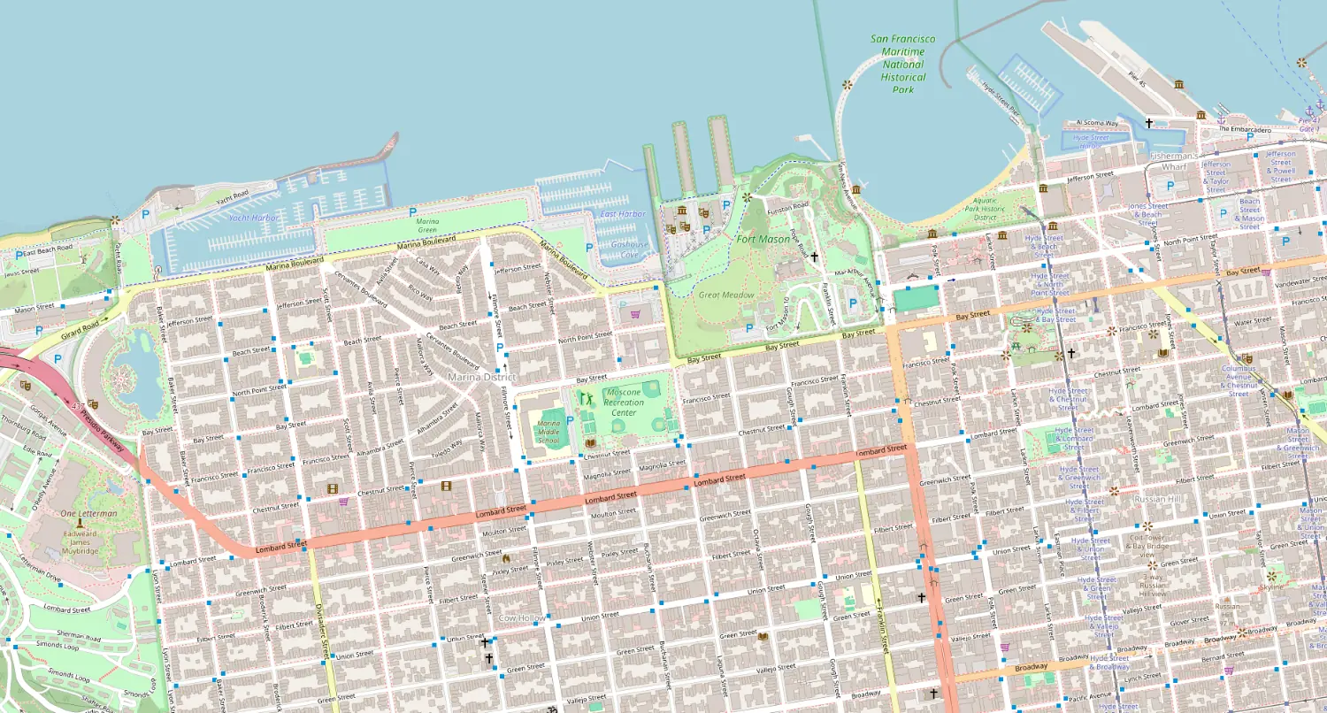
Start Georeferencing then wrote the GeoTIFF in 34 seconds and added it to the project. On OpenStreetMap, the 1947 streets land on today's:
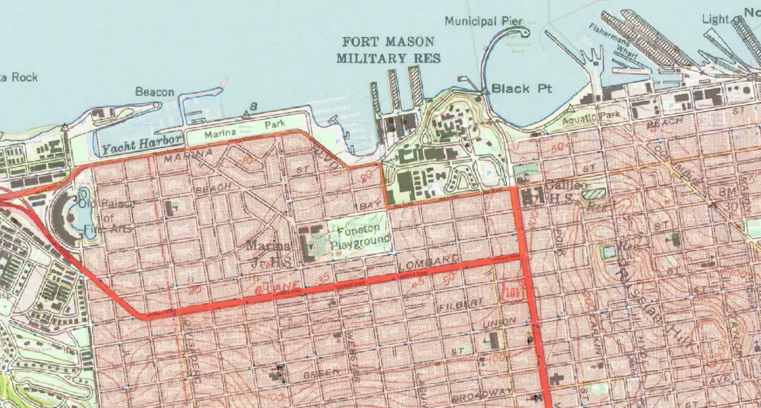
Use it when: you want a result you can defend, with residuals, a .points file and a GeoTIFF any GIS reads.
Skip it when: you only need a rough backdrop for a few minutes. Method 2 is faster for that.
Method 2: A freehand overlay with a plugin
The Freehand raster georeferencer plugin, version 0.8.3 when I read its documentation, lets you drop an image on the map and move, rotate and scale it by hand until it lines up, the way you would in Google Earth. The result shows on top of your other layers at once, and the plugin exports the image with a world file when you are done.
Its README is clear about the limits: affine transformations only, no rubber sheeting, no residuals, and only BMP, JPEG, PNG and TIFF files. You get no number that says how far off you are.
Use it when: you need a scanned plan roughly in place to trace a few features or to show a client where things were.
Skip it when: anyone will measure on the result. Use Method 1.
Method 3: Control points checked by an AI agent
We build AI Agent, a free QGIS plugin with a chat panel that runs the steps in your open project. This section is about our own tool. It has a georeferencing tool that takes control points as pixel and coordinate pairs, fits one of the Georeferencer's transforms through GDAL, and returns each point's residual in metres judged against the map's scale.
It can also place a scan with no points at all, by reading its place names and matching it against reference maps: an old map of Edinburgh in the AI Agent guide landed with a 5.9 m median error. That needs readable names, and very old sheets often fail. For a map with a printed graticule, the points are the surer route, and reading them is quick: an image with no coordinates sits in QGIS with the pixel column as x and minus the row as y, so the status bar shows the pixel under your cursor. I loaded the scan, kept the typo from the test above in point 8, and sent one message:
Georeference the layer sf-north-1947-scan. It is the USGS San Francisco North quad from 1947, scale 1:24,000, coordinates in NAD27. I read these control points on the scan (pixel column, row → latitude, longitude): 1. 1022, 792 → 37°52'30"N, 122°30'W (NW corner) [...] 8. 4632, 5344 → 37°47'N, 122°25'W. Is the result accurate enough for a 1:24,000 map?
The run took 99 seconds, shown in the panel as 14 actions. The agent read the layer, fitted the eight points in Python to check them, found that point 8 sat 925 m from where its row put it, left it out, and wrote the GeoTIFF from the other seven in NAD27 / UTM zone 10N.
It asked once, before running its own Python check. Its answer gave an RMSE of 0.73 m with a 0.95 m maximum against a 4.8 m tolerance, and added that this measures agreement between points, not the map's absolute accuracy.
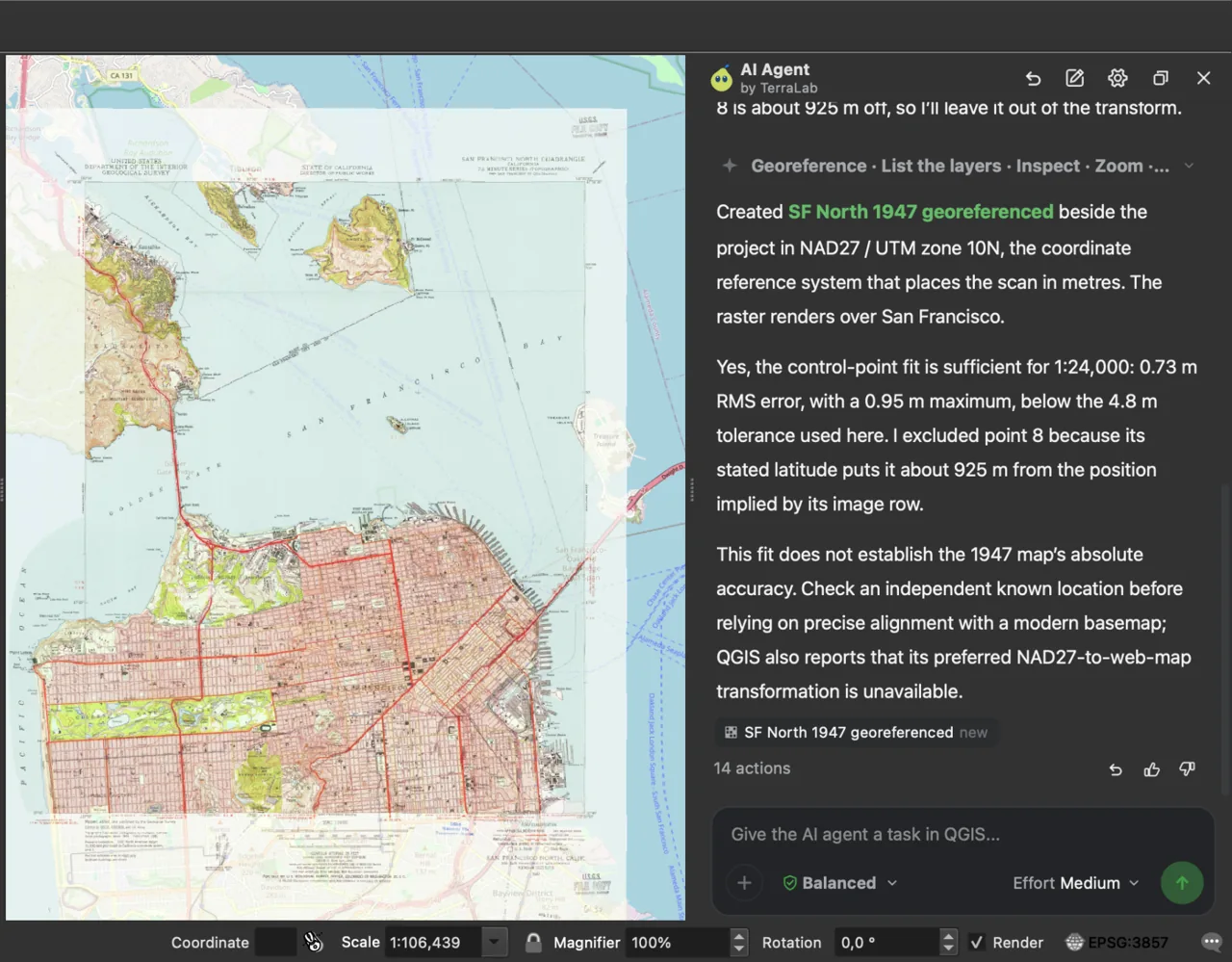
I checked its GeoTIFF the same way as mine, on the eight edge ticks it never saw: 1.0 m off on average, 1.6 m at worst, the same as the Georeferencer. The difference is the typo. In the Georeferencer I would have had to spot it in the residual column myself, and with a thin plate spline I would not have spotted it at all.
It also left the points behind as a .points file next to the output, so the same fit opens in the Georeferencer if you want to move a point by hand. Each message leaves a checkpoint in the panel, and one click undoes the whole run. The free plan has 10 messages a month with no API key and no card.
Use it when: you have the points and want the fit, the outlier check and the verdict in one step, or you georeference sheets in a series.
Skip it when: the map has neither readable place names nor points you can read, such as a hand-drawn sketch. Placing points by hand in Method 1 is then the only route.
What to remember
- In QGIS 3.26 and later the tool is
Layer > Georeferencer. Start with four well-spread points, Polynomial 1 and a projected target CRS on the map's own datum. - An RMSE of zero proves nothing: a thin plate spline always reaches it, and in my test it did so on a map 594 m off.
- Convert residuals to metres (pixels x ground size of one pixel) and compare them with what the map promises, 12.2 m for a 1:24,000 USGS sheet.
- Check the result on points you left out of the fit. Mine were 1.0 m off on average on the 1947 San Francisco sheet.
- Type the points in the datum the collar names. NAD27 sits 93 m from WGS 84 in San Francisco, so a 1947 USGS sheet takes EPSG:4267.
Questions people ask
Where is the Georeferencer in QGIS?
In QGIS 3.26 and later it is under Layer > Georeferencer. In older versions it was Raster > Georeferencer, provided by the GDAL Georeferencer plugin, which had to be enabled in the plugin manager. If neither menu shows it, a plugin or a customization profile may have changed your menus.
How many control points do I need?
The minimum is 2 for Linear and Helmert, 3 for Polynomial 1, 4 for Projective, 6 for Polynomial 2 and 10 for Polynomial 3, and the QGIS manual asks for 10 or more for a thin plate spline. In practice use about twice the minimum, spread to the corners, and keep a few more aside as checkpoints. I used 8 for Polynomial 1 and 8 more to check.
Polynomial, Helmert or thin plate spline: which one?
Helmert for a clean, flat scan that only needs rotating and scaling. Polynomial 1 for almost every printed map, since it also absorbs a small shear from the scanner. Thin plate spline only for a damaged or hand-drawn map with many good points, and then check it on points you did not use, because its residuals are always zero.
What is a good RMSE?
One that is small next to what the map can deliver. Convert it to metres and compare it with 0.2 mm times the scale denominator (4.8 m at 1:24,000) or with the map's official standard (12.2 m for USGS 1:24,000 sheets). Under one pixel on a clean scan is normal. A single point with a residual far above the others is usually a typo or a wrong click, not a bad map.
How do I georeference a PDF?
First check whether it already is. USGS topographic maps and many agency plans are GeoPDFs, and QGIS opens them in place: the 1947 San Francisco PDF loaded with its coordinates and no control points, rendered by GDAL at 150 dpi unless you set GDAL_PDF_DPI higher. A plain PDF has no coordinates: export the page to PNG or TIFF at 300 dpi, then use Method 1.
How do I georeference a map with no coordinates on it?
Use features that have not moved since the map was drawn, such as road intersections, bridges, churches and coastline corners, and pick their coordinates with From Map Canvas on a basemap or on your national orthophoto. Spread 10 or more of them across the sheet. Expect larger residuals than with a printed grid, because the old map and today's world no longer agree everywhere.
The QGIS AI hub collects what AI can and cannot do inside QGIS, and the AI Agent guide covers the rest of the plugin. Once the old map is in place, you can download OpenStreetMap data to compare it with today's streets, pull a Sentinel-2 image of the same area, or turn the scan into vectors.