Detect Building Footprints in QGIS: 3 Methods
Published Updated
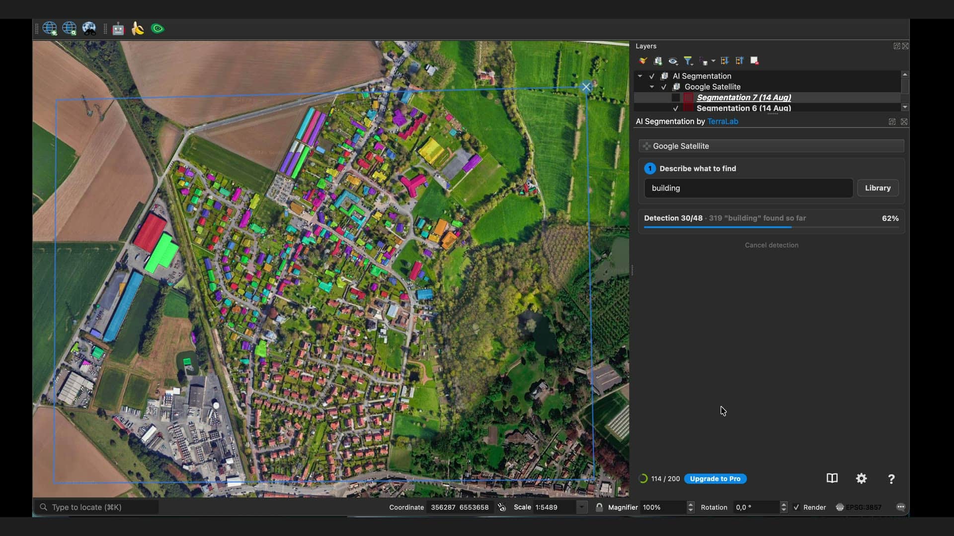
To detect building footprints in QGIS you have three routes: download an open dataset, run an AI detection plugin over your own imagery, or digitize by hand. The fast one is the second. Install the plugin from the plugin manager, load your imagery, draw a zone, type buildings, hit Detect, and a polygon layer lands in your project CRS.
 you have three routes: download an open dataset, run an AI detection plugin over your own imagery, or digitize by hand. The fast one is the second. Install the plugin from the plugin manager, load your imagery, draw a zone, type
 Filtering is the second half of the job. A large share of what comes back is not a building, so cut the raw output by confidence and area. I ran one pass over central Paris, got 635 polygons, and deciding which 82 to keep took longer than the detection did.
| Your input | Method | Time |
|---|---|---|
| An area OpenStreetMap, Microsoft or Google already cover | Method 1: download open footprints | Minutes |
| Hundreds to thousands of buildings, on the exact imagery you were handed | Method 2: automatic detection (ours, cloud) | 848 buildings in 57 seconds, then the filtering |
| Under fifty buildings, or a historic centre where you need one polygon per address | Method 3: digitize by hand | As long as it takes you |
Open data first, every time. You only move on when the coverage has holes, the vintage is wrong, or the footprints have to match the specific orthophoto a client handed you.
Method 1: Download open footprints
You need QGIS 3.22 or newer, one imagery layer you trust, and an internet connection for method 2. No dedicated graphics card, on any of the three.
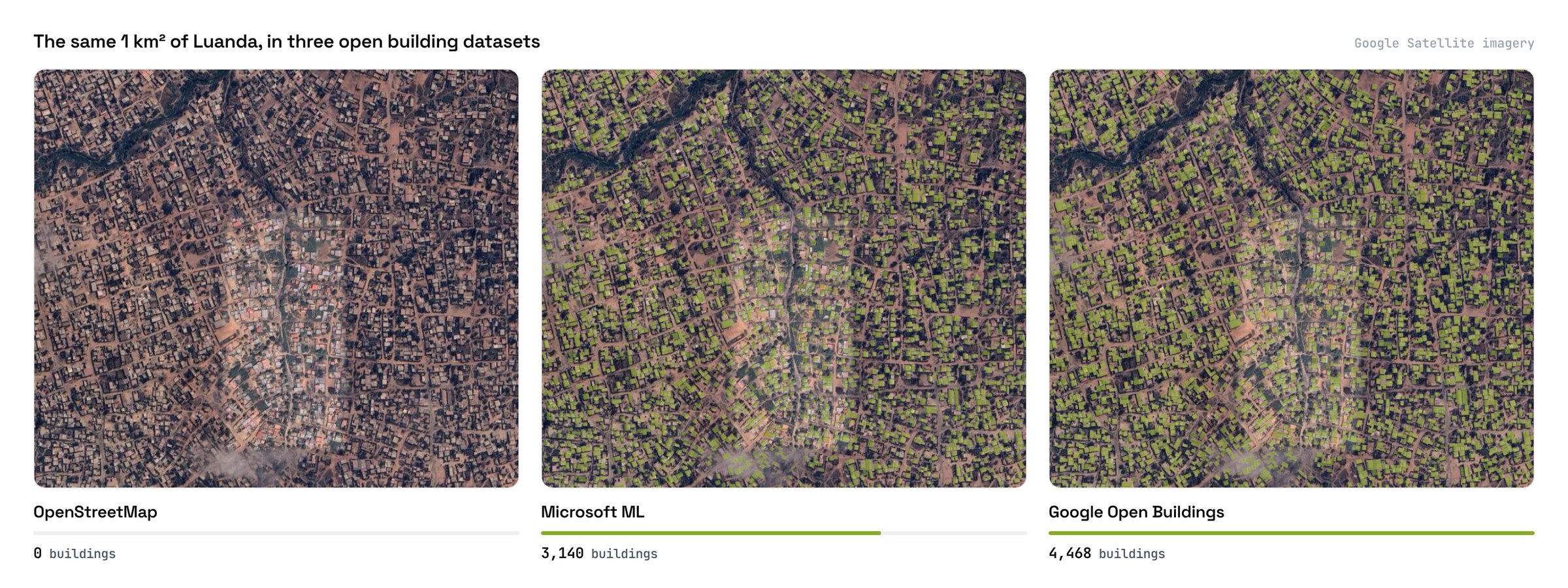
For a lot of jobs you don't need to detect anything. Three open datasets cover most of the planet between them, and over one neighbourhood they can disagree by thousands of buildings.
Pick the dataset for your area
OpenStreetMap is excellent wherever mappers are active, and buildings carry attributes. Microsoft Global ML Building Footprints holds over a billion machine-extracted buildings and is strongest in North America. Google Open Buildings covers the Global South, where OSM is thinnest. To see what each of them holds for your area before loading anything, draw a box in our free building footprint downloader and download the one you want as GeoJSON.
Load one against your imagery
Pull OSM in with QuickOSM.
Zoom in and look at the edges
That one look decides whether you stop here or read on.
Use it when: the area is already mapped well and you can live with the dataset's vintage and licence.
Skip it when: the coverage has holes, the vintage is wrong, or the footprints have to line up with one specific orthophoto.
Method 2: Automatic detection
A building footprint is the outline of a building where it meets the ground, as a flat polygon. Not the roof, not the parcel, not the address point. Which matters here, because vertical imagery gives you the roof: on a five-storey Haussmann block shot near-nadir the offset is small, on a tower it is not. Worth knowing before you promise anyone a footprint layer, and there is a longer version in what a building footprint is.
An automatic detection model reads your imagery and returns building outlines as polygons, each with a confidence score. We build one of these, AI Segmentation. This section is about our own tool.
It installs from the plugin manager like any other: no download by hand, no Python environment, no dedicated graphics card, because the model runs on our servers. Windows, macOS and Linux.
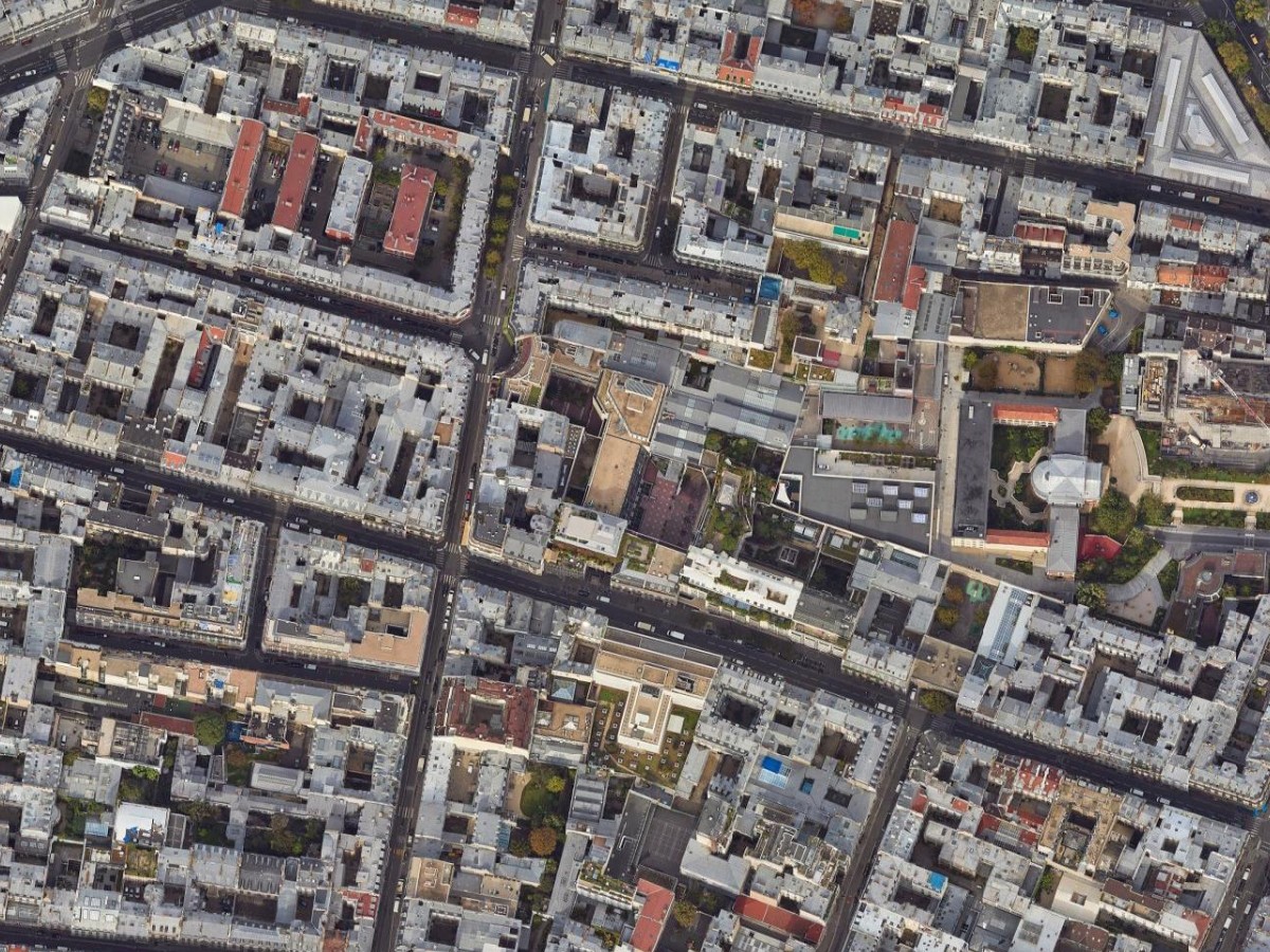
Install it and pick your imagery layer
Plugin manager, install, open the panel, choose the raster you want read.
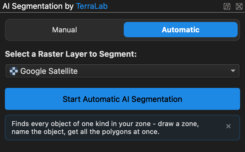
Draw a zone and name the object
Draw a zone, type buildings, hit Detect. That's the whole prompt, in your own language if you prefer. Results stream back tile by tile as one polygon layer in the project CRS.
Set the precision when the objects are small
The one setting worth learning is precision, which is the tile size. Small tiles give the model a close look, which small objects need. Big tiles give it context, which a farm parcel needs.
Filter what came back
The panel walks you through three steps before anything becomes a layer: filter what to Keep, Correct what the model missed, and choose the output Shapes. The first one is where the job is won, and it gets its own section below.
Clean the geometry
Simplify, orthogonalize and delete holes, in that order, and only where each earns its place. The three tools and the reason for the order are below.
A run counts the ground it covers. Every account gets a free allowance each month, no card asked for, and Pro raises it. Detection runs on European servers, we do not train on your imagery, and there is a small local model if nothing may leave your machine. The complete guide covers Keep, Correct and Shapes in full.
Filtering is the whole job
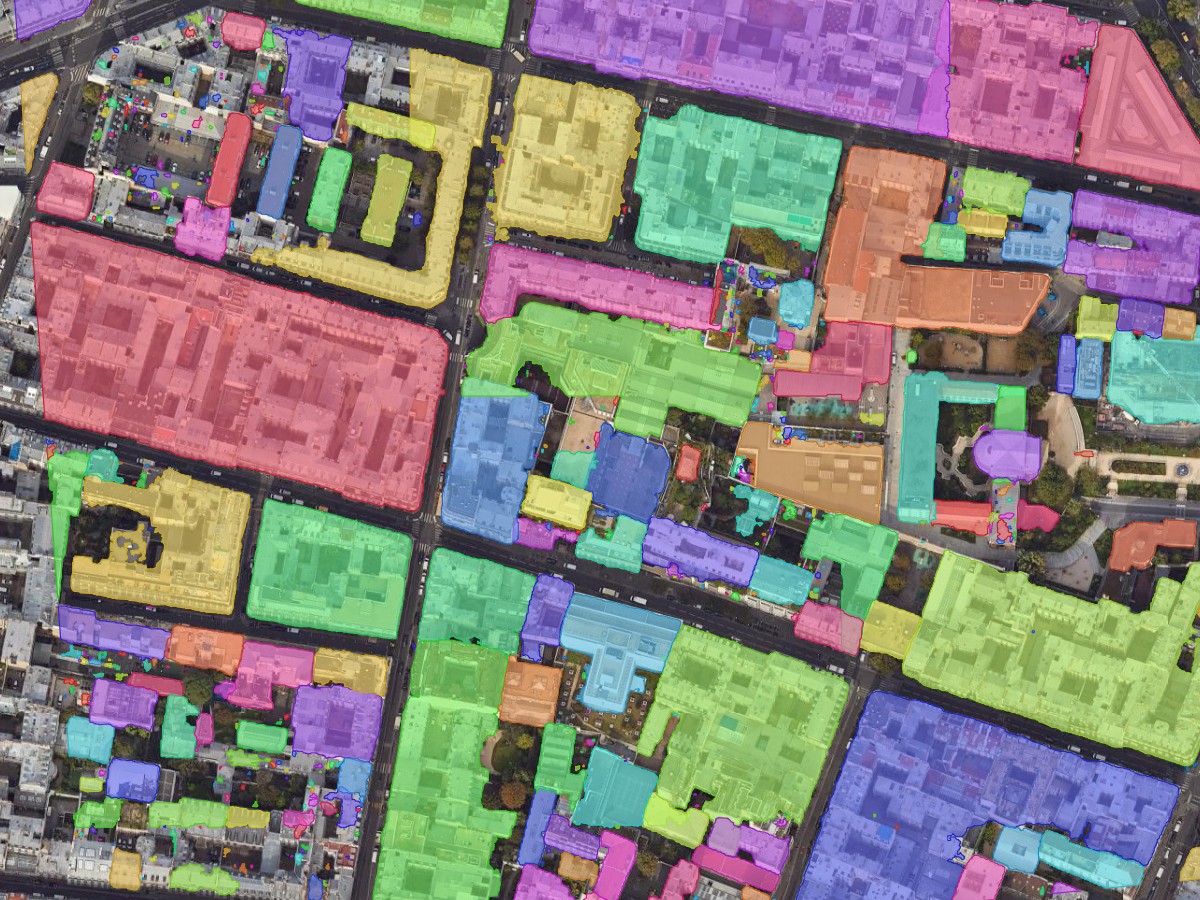
Raw detection output is a set of candidate polygons with confidence scores. On dense imagery most are small and uncertain. I exported this Paris run with both filters wide open, so every candidate landed in the layer: 635 polygons over 1.18 km².
Half of what came back is smaller than a parking space: vents, skylights, stairwell housings, courtyard sheds. Real things on the imagery, correctly outlined, and not what anyone means by a building footprint.
So filter. Move the two sliders in the panel, or do the same job from the attribute table with Select by Expression:
"area_m2" >= 50 AND "score" >= 0.5
That leaves 82 polygons out of 635, covering 222,338 m² of the 263,658 m² total. Rather than take my word for the thresholds, move them yourself. Green survives your filter, white does not.
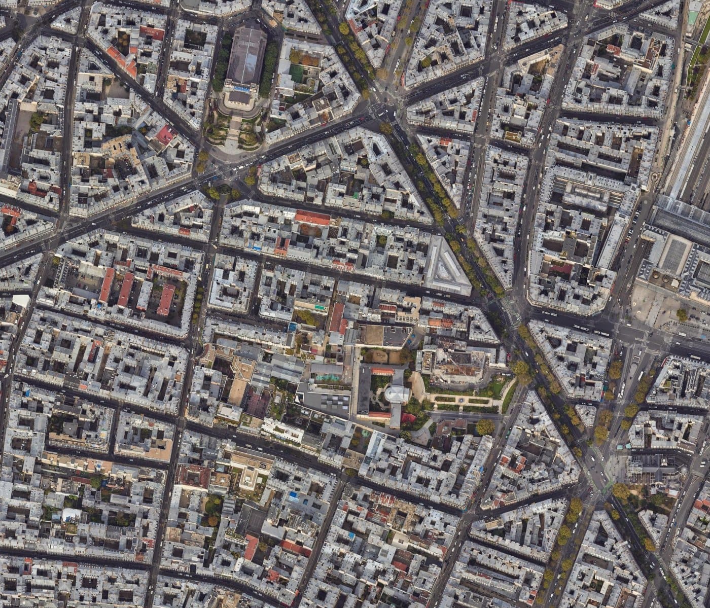
82 / 635polygons kept (13%)
84%of the built area (222,338 m²)
The same 635 detections the attribute table holds. Drop the confidence to zero and the courtyard sheds and skylights come back.
Watch the second number while you drag the first. Throwing away 87% of the polygons costs 16% of the area, and the rest is noise you'd have deleted by hand anyway, one at a time, while wondering whether the tool was any good.
Tune both to the job. A survey of industrial sheds can push the area floor to 200 m². Mapping informal settlements, 50 m² throws away real houses, so drop to 15 and lean on the confidence score instead.
What a clean result looks like
Paris is a hard case. Same tool on detached housing about 10 km west:
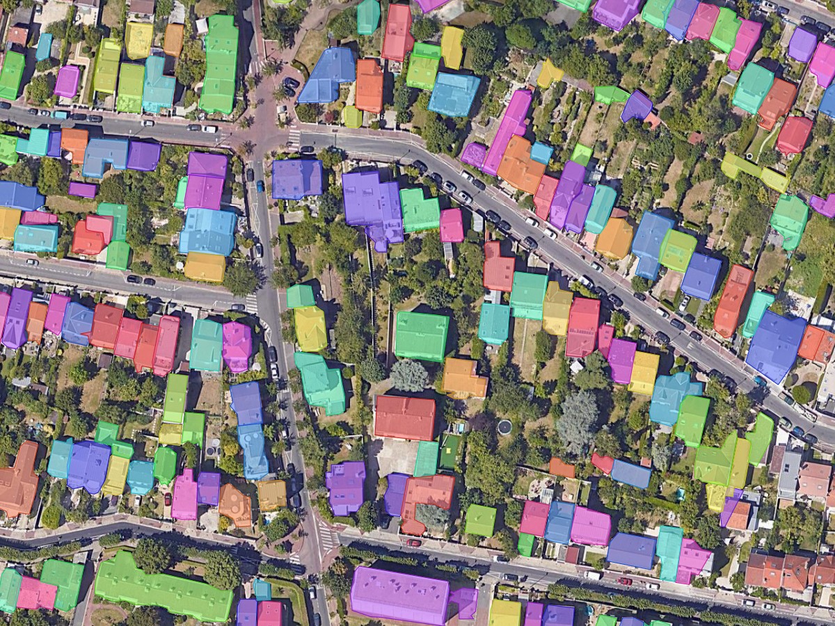
85m²
median polygon area
Paris run: 3.2 m²
0.79
median confidence
Paris run: 0.26
251polygons
kept, out of 251 returned
Paris run: 82 out of 635
Same tool, same city, nothing to throw away. What changed is the built fabric, not the model.
Where it breaks: dense continuous blocks
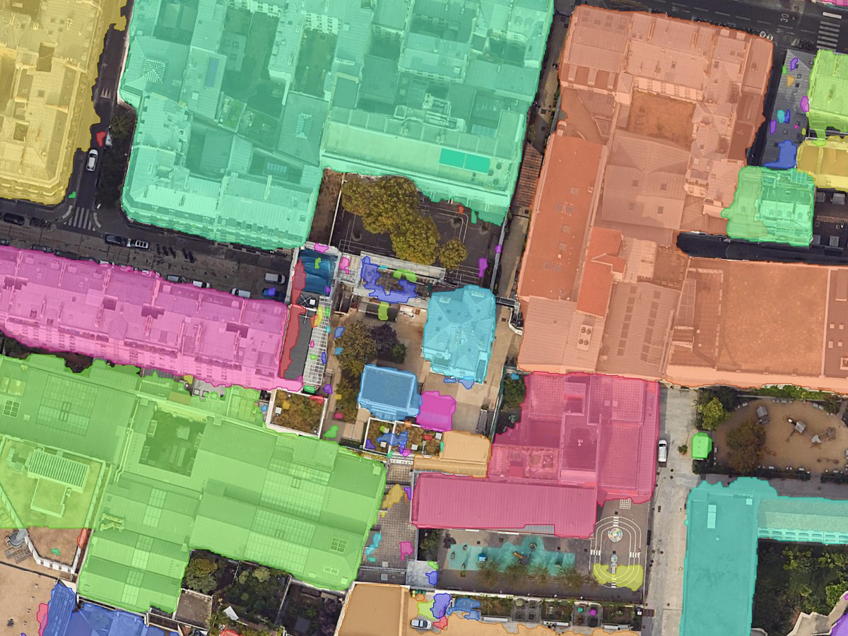
Each polygon traces the built envelope of a whole block, hugging the street line and correctly cutting out the courtyards. Good for built-up area or impervious surface, wrong if you need a polygon per address. No model reading a vertical image can find the party wall between two attached buildings, because from above there is nothing there to see.
Cleaning the geometry
Three native QGIS tools tidy a footprint layer, and the order matters because simplify moves the vertices you just squared.
- Simplify, 0.5 m tolerance over aerial imagery. Cuts the vertex count hard without moving the boundary anywhere you'd notice.
- Orthogonalize. Snaps near-right angles square. Reach for it on open data or hand-traced work, where nothing has squared them yet.
- Delete holes, only if you want solid footprints. Not on the Paris result: those holes are courtyards and they're correct.
On a detected layer step 2 is close to a no-op. I measured that rather than assume it, running Orthogonalize over 190 detected buildings and comparing all 1,845 corners before and after.
87.9%
corners already within 1° of square
before running anything
87.9%
after Orthogonalize
the same 1,845 corners
1.7cm
median vertex shift
9.1 cm at the worst
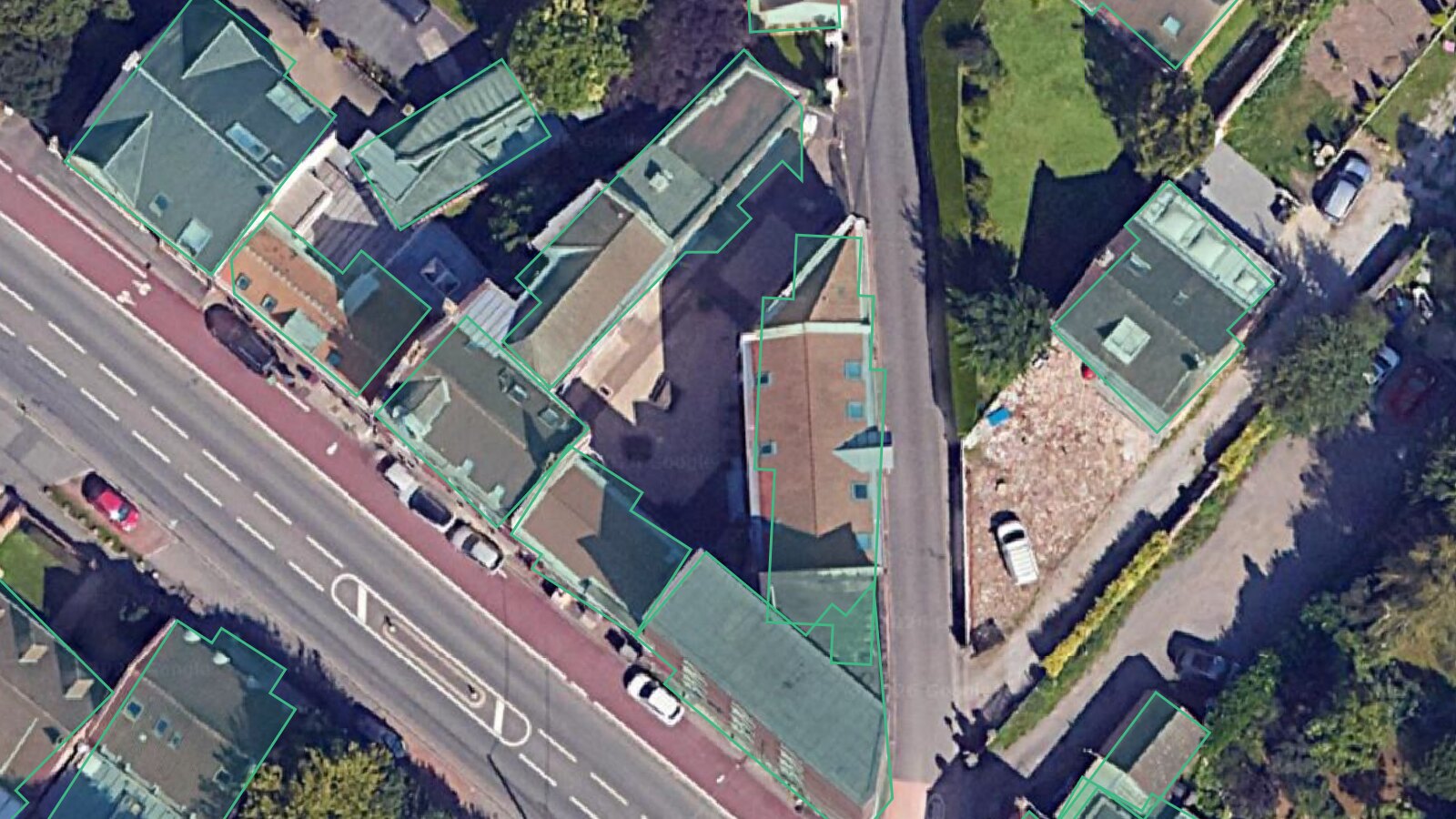
The 12% that are not square are the attached terraces. Look at the stepped edge running down the middle of the block. No corner tool fixes that, because those steps follow a real roof line rather than a modelling error.
Use it when: hundreds to thousands of buildings, on imagery you have to match, or when several people must produce the same layer the same way.
Skip it when: you need a polygon per address in a historic city centre. I wouldn't use automatic detection for that, and cadastral data plus manual correction wins there.
Try it free in QGIS, no card needed
Method 3: Digitize by hand
Under fifty buildings, draw them. Free, exact, and I'd still do it myself at that size.
Turn on snapping
Project -> Snapping Options, vertex and segment, topological editing on. Skip it and you'll spend the afternoon deleting slivers.
Trace, and watch yourself drift
Around the 60th building you start cutting corners you'd never have cut on the 6th, and you don't notice. It's already in the layer.
Use it when: under about fifty buildings, or when you need one polygon per address in a dense historic centre.
Skip it when: the count runs into the hundreds, or several people have to produce the same layer the same way.
What to remember
| Open datasets | Automatic detection | Hand-digitizing | |
|---|---|---|---|
| Cost | Free | Free tier, then paid | Free |
| Setup | Minutes | Minutes | None |
| Good for | Areas already covered well | Hundreds to thousands | Under ~50 buildings |
| Matches your imagery | No | Yes | Yes |
| Consistent across a team | Yes | Yes | No |
| Dense continuous blocks | Varies | Block envelopes only | Yes |
| Provenance you can state | Dataset and vintage | Your imagery, with a confidence score | You |
Check the open datasets first. Over one neighbourhood they disagree by thousands of buildings, so one look at their edges against your imagery decides whether you go further.
Footprints that have to line up with a client's orthophoto rule out the open datasets, whatever their coverage.
Filtering a detection is most of the work: 82 polygons out of 635 over central Paris, holding 84% of the built area.
A vertical image cannot give you one polygon per address where buildings touch, at any price. Join to cadastral data instead.
Past about fifty buildings, hand-digitizing drifts without telling you.
Questions people ask
Does it work on drone imagery?
Better than on satellite. Ground resolution matters more than the source: a 5 cm orthophoto gives cleaner boundaries and higher confidence than a 30 cm satellite scene.
Do I need a GPU?
What does a run cost?
Automatic counts the ground your zone covers, and Cloud AI counts one object per save. Semi-Auto on your own machine is free. Every account gets a free allowance each month.
Can I get one polygon per address?
Not from a vertical image, in a city centre where the buildings touch. The model returns the built envelope of the whole block, courtyards cut out, which is right for built-up area and wrong for addresses. Join to cadastral data instead.
Which open dataset should I start with?
OpenStreetMap, if your area has active mappers. Where it doesn't, the gap is stark: over that 1 km² of Luanda OSM maps no buildings at all, while Microsoft finds 3,140 and Google Open Buildings 4,468.
For the roof-versus-ground gap in full, read what a building footprint is. For the classified-raster case, where polygonize beats any model, read raster to vector in QGIS. The same zone-and-filter method finds the panels on those roofs: solar panel detection in QGIS walks through it. For running this detection and filtering sequence on a new area without repeating each click, AI Agent does it from one instruction in QGIS. A brownfield site often shows up in the detection as leftover slabs and sheds rather than clean roofs, and the greenfield vs brownfield page covers how each looks from the air. The QGIS AI hub lists the rest of what we build.