How to Download Sentinel-2 Images in QGIS

Centre-pivot farms near Cristalina, Brazil, on 7 July 2026, true colour on the left and NDVI on the right, the two halves meeting across the same circles. — Centre pivots near Cristalina, Brazil, 7 July 2026. Left, true colour. Right, NDVI from the same Sentinel-2 scene. Contains modified Copernicus Sentinel data 2026.

To get Sentinel-2 images into QGIS 3.42 or newer, open Layer > Data Source Manager, pick the STAC tab and add a connection to Earth Search, https://earth-search.aws.element84.com/v1. Filter by extent, dates and the Sentinel-2 Level-2A collection, then right-click a scene and choose Add Layer > True color image. The image streams in without an account or a download.

When you do want the file itself, the full product in .SAFE format, Copernicus Browser is the official source and asks for a free account. I ran every method below on 23 September 2026 in QGIS 3.44.7, on the centre-pivot farms around Cristalina, in the Brazilian state of Goiás, and timed each one.

The short answer

You want	Method	Measured on Cristalina
The full product on disk, every band and the metadata	Method 1: Copernicus Browser	About 1.1 GB per scene, free account
An image on the map now, then true colour and NDVI	Method 2: STAC in the Data Source Manager	5.4 s to draw 133 km² at 10 m, no account
Scenes for a classification you will run in SCP	Method 3: Semi-Automatic Classification Plugin	26 s to search, extra Python packages to install
The least cloudy scene and an NDVI layer in one message	Method 4: an AI agent in QGIS	2 min 47 s, 35 actions

My default is Method 2. In 2026 you rarely need to download a Sentinel-2 scene to look at it or to compute an index on a few fields. Download the product when you need all 13 bands offline or an archive you control.

Before you start

Sentinel-2 is the European Copernicus optical mission. In July 2026 three satellites, Sentinel-2A, 2B and 2C, were all acquiring: the catalogue holds 9 dates over Cristalina that month. Each scene is cut into tiles of 109.8 km by 109.8 km in UTM, named like 22KHG, and a place near a tile edge sits on two tiles. Cristalina sits on 22KHG and 23KKB.

Two processing levels matter. Level-1C is reflectance at the top of the atmosphere. Level-2A is corrected for the atmosphere into surface reflectance and ships a scene classification band (SCL) that flags cloud and shadow. For anything you compare across dates, NDVI included, take L2A.

The bands you will use most are 10 m: B2 blue, B3 green, B4 red and B8 near infrared. True colour is B4, B3, B2 as red, green, blue, and NDVI is (B8 − B4) / (B8 + B4), the two definitions Copernicus Browser prints under its own layers. The multispectral vs hyperspectral post explains what the other bands measure.

You need QGIS 3.40 or newer for STAC in the Browser panel and 3.42 or newer for the search in the Data Source Manager, per the 3.40 and 3.42 changelogs.

Where the web gets this wrong

"You have to download the product first." Most tutorials still start with a 1 GB zip. Earth Search and other STAC catalogues serve every Sentinel-2 L2A band as a Cloud-Optimized GeoTIFF, and QGIS reads only the part of the file it draws. The true colour file for the Cristalina tile is 297 MB. QGIS drew my 133 km² window from it at full resolution in 5.4 seconds, cold, without saving anything.

"NDVI is (B8 − B4) / (B8 + B4) on the raw values." Since processing baseline 04.00, deployed on 25 January 2022, L2A values carry an offset: reflectance is (value − 1000) / 10000, and MTD_MSIL2A.xml says so with BOA_ADD_OFFSET -1000. On raw values the formula is wrong. On one window of the same pivot I got 0.517 from raw numbers and 0.768 once the offset was removed.

The catch is that some sources fix the offset for you. The .SAFE JP2 bands don't, and QGIS reads them as raw numbers. The Earth Search Collection 1 COGs carry a scale and an offset that QGIS applies on load, so there the plain formula is right. Click one pixel with the Identify tool first: thousands mean raw numbers, values between 0 and about 1 mean reflectance.

"The cloud percentage is the cloud over your field." It is the cloud over the whole tile. On 29 July 2026 the same satellite pass over Cristalina reads 22% cloud on tile 22KHG and 2.6% on tile 23KKB. A 20% scene can be clear over your farm, and a 3% one can have its only cloud on it. Look at the image, or at the SCL band, over your own area.

Method 1: Download the L2A product from Copernicus Browser

Copernicus Browser is the official front door to the archive. You can search without an account. The download asks you to log in, and registration is free.

Open the Search tab. Tick SENTINEL-2, then L2A, and drag the cloud slider down to 10%. Set the time range, and mark a point of interest or draw an area on the map. Click Search.

Pick a scene

For July 2026 over Cristalina the Browser listed 9 L2A products under 10% cloud, out of 18 that month. Each one is a .SAFE product of about 1,090 MB, one per tile and date. Use the small thumbnail to judge the cloud over your area.

Download

Click the download arrow. Anonymously, the Browser answers "You need to log in to use this function." Log in and the zip downloads.

Load the bands in QGIS

Unzip it. The 10 m bands are in GRANULE/<granule>/IMG_DATA/R10m/ as JPEG 2000 files, one per band, about 105 to 130 MB each. TCI_10m.jp2 is a ready-made 8-bit true colour image: drag it onto the map.

Build your own composite

For your own stretch, run Raster > Miscellaneous > Build Virtual Raster… on B04, B03 and B02, in that order, with "Place each input file into a separate band" ticked. For NDVI, apply the offset in the Raster Calculator: ("B08" - "B04") / ("B08" + "B04" - 2000).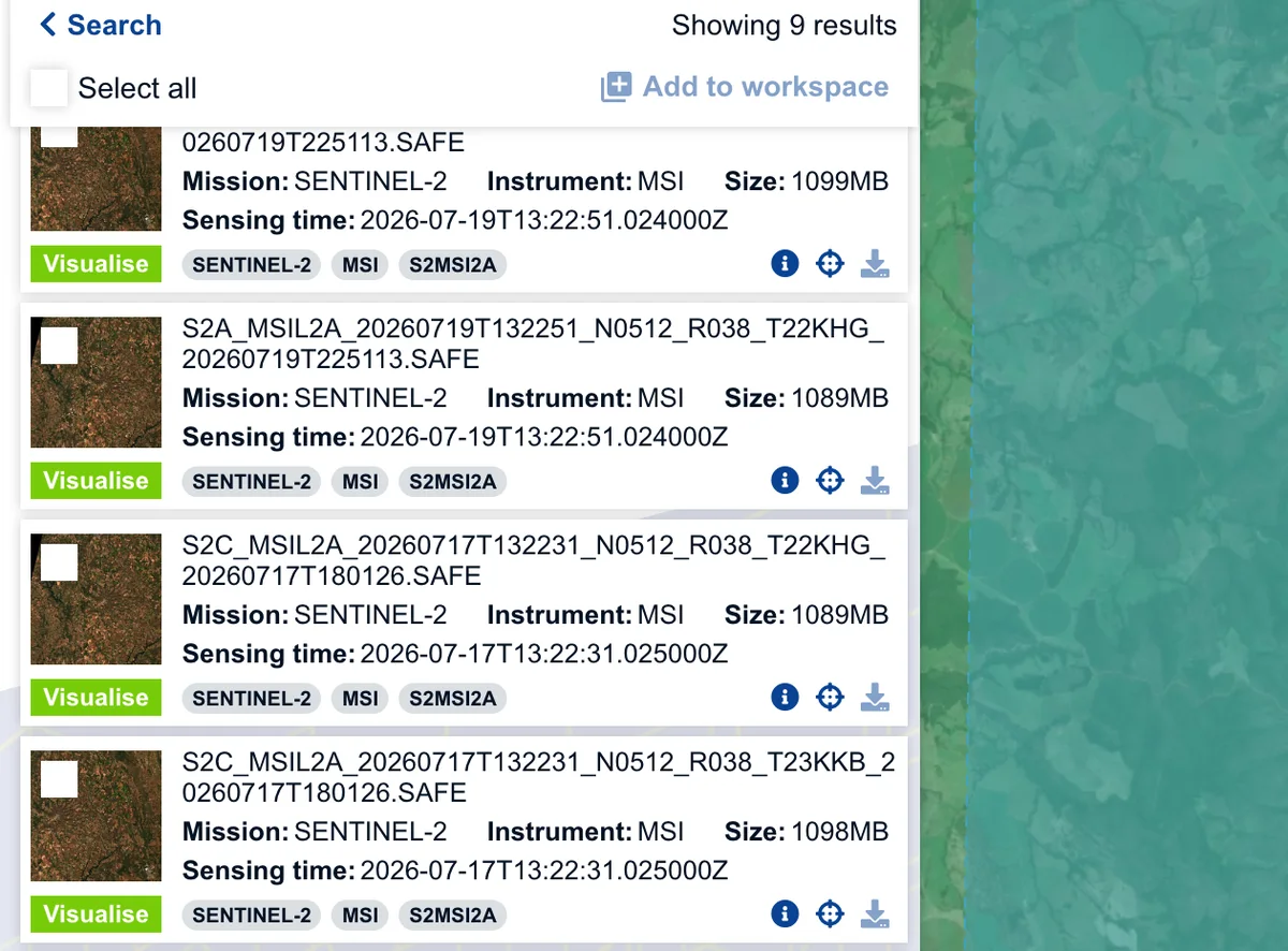

Copernicus Browser search results for Sentinel-2 L2A over Cristalina in July 2026, each product with its name, size of about 1,090 MB, sensing time and a download arrow. — Copernicus Browser v1.56.0, 23 September 2026: 9 L2A products under 10% cloud for July 2026. Sizes run from 1,088 to 1,101 MB, one product per tile and date.

Use it when: you need every band offline, the metadata and quality masks, or an archive that does not depend on someone else's server.

Skip it when: you only need to see a place or compute an index on a few fields. You would download 1.1 GB to use a few megabytes of it.

Method 2: Stream it with STAC in QGIS

STAC is the catalogue standard most satellite archives now publish. QGIS reads it natively, and Earth Search by Element 84 serves Sentinel-2 L2A from the AWS open data bucket with no key.

Microsoft Planetary Computer has the same archive, but its files need a signed token: an unsigned request for the 7 July image returned HTTP 409, and my QGIS 3.44.7 build has no authentication method for it. So I used Earth Search.

Add the connection

Layer > Data Source Manager, STAC tab, New. Name it, paste https://earth-search.aws.element84.com/v1, OK, then Connect.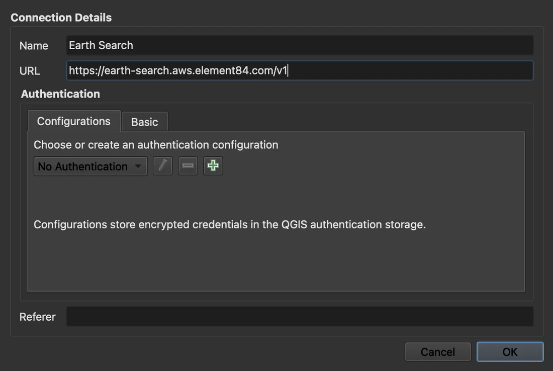

The QGIS STAC Connection dialog with the name Earth Search, the URL https://earth-search.aws.element84.com/v1 and No Authentication. — One connection, no authentication. It stays in your QGIS profile for the next project.

Set the filters

Click Filters…. Tick Spatial Extent and take it from the map canvas or a layer, tick Temporal Extent and set the dates, then keep only "Sentinel-2 Collection 1 Level-2A" in the collection list. OK runs the search.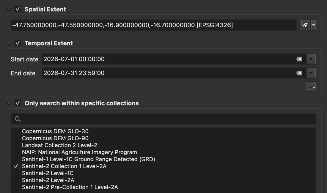

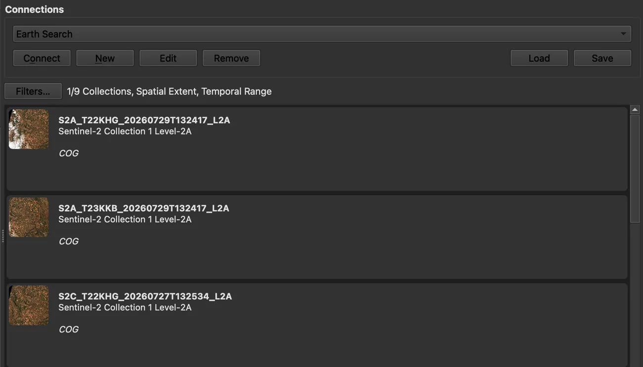
The QGIS STAC Search Filters dialog: a spatial extent in EPSG:4326 around Cristalina, dates from 1 to 31 July 2026, and only Sentinel-2 Collection 1 Level-2A ticked. — Extent, dates, collection. There is no cloud cover filter in QGIS 3.44.

The search returned the same 18 scenes as the Copernicus catalogue. Each row carries a thumbnail, and the thumbnail is your cloud filter: the first row, 29 July on tile 22KHG, shows its cloud before you open it. Double-click a row for Details…, where eo:cloud_cover gives the tile percentage.

STAC search results in the QGIS Data Source Manager: Sentinel-2 Collection 1 Level-2A scenes from July 2026, each with a thumbnail and the label COG. — Results arrive newest first, with a thumbnail and the COG label. The white patches on the first thumbnail are cloud.

Add only the bands you need

Right-click the scene, Add Layer, then True color image. Repeat for Red - 10m and NIR 1 - 10m if you want NDVI. The Add button at the bottom loads every streamable asset of the scene at once, which is rarely what you want.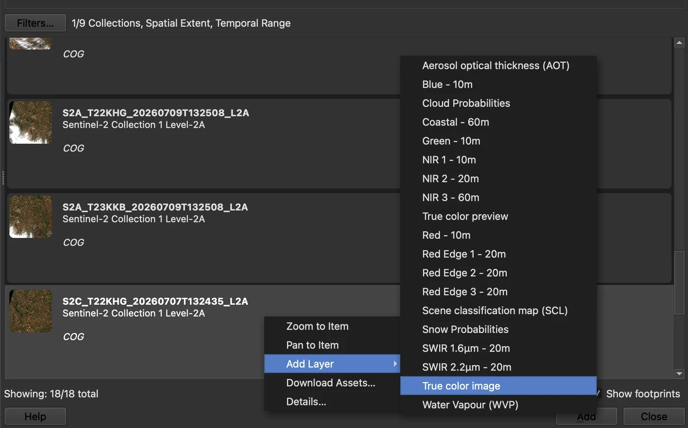

The right-click menu on the 7 July 2026 scene in the QGIS STAC results, with Add Layer open on the list of assets and True color image highlighted. — Right-click, Add Layer: one entry per band. The two menus are captured from the running QGIS and placed where Qt draws them.

The layers load as /vsicurl/ links to the COG files. Pan and zoom, and QGIS fetches the tiles it needs at the level of detail it needs. The legend tells you the second thing worth knowing: the red band reads from about 0 to 1.6, not in thousands, because QGIS applied the file's scale and offset.

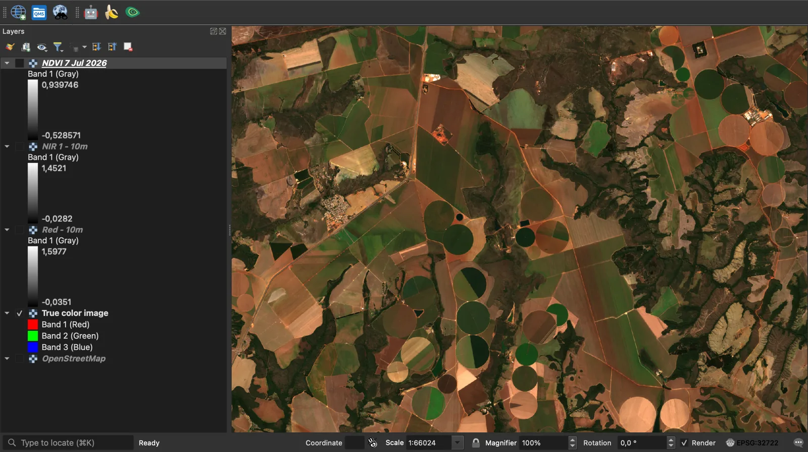
QGIS with the Sentinel-2 true colour image of 7 July 2026 over the Cristalina pivots, and the Layers panel listing the true colour, red, NIR and NDVI layers, the red band legend reading -0.0351 to 1.5977. — Streamed, not downloaded. The red and NIR legends are in reflectance, so the plain NDVI formula applies.

Compute NDVI

Raster > Raster Calculator…, expression ("NIR 1 - 10m@1" - "Red - 10m@1") / ("NIR 1 - 10m@1" + "Red - 10m@1"). Set the extent to your area, not the whole tile: I used 11.4 by 11.6 km around the pivots, 1,140 by 1,163 pixels at 10 m. It wrote the GeoTIFF in under a second.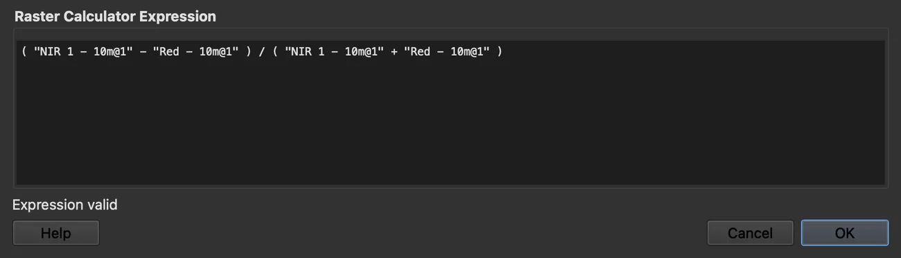

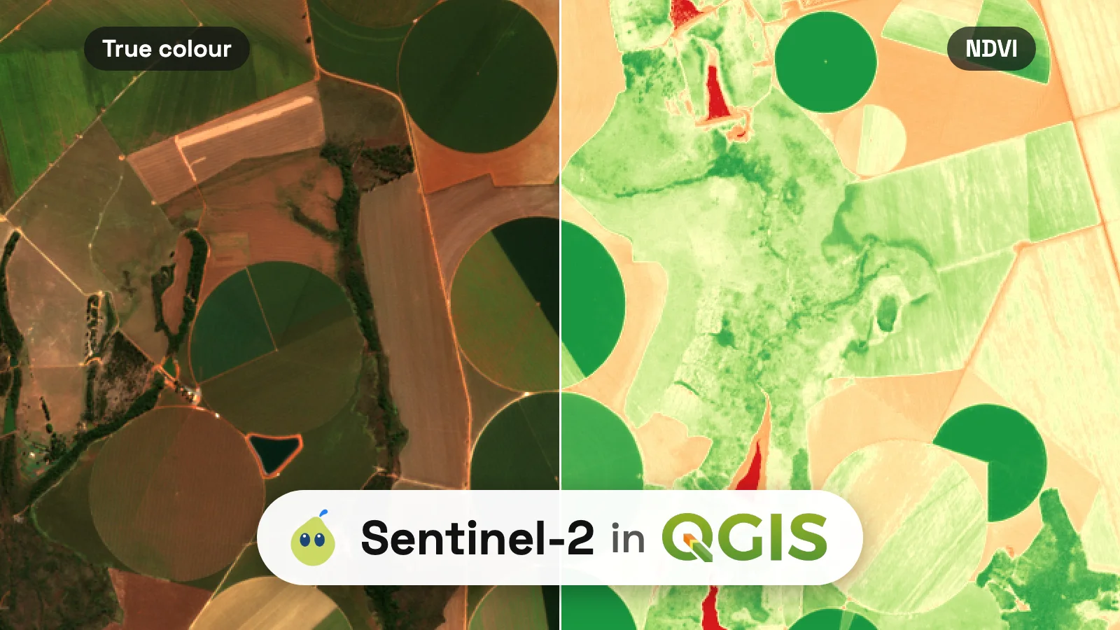
The QGIS Raster Calculator expression box with the NDVI formula on the NIR 1 and Red layers, marked Expression valid. — No offset term here, because these COGs already arrive as reflectance.

My NDVI ran from −0.65 over the farm ponds to 0.94 on the irrigated circles, with a mean of 0.48. It matched the AI Agent's layer in Method 4 pixel for pixel. July is the dry season on this plateau: the pivots that are growing sit at 0.85 to 0.93, bare fields at 0.2 to 0.3. In true colour a growing pivot and the dark gallery forest along the streams look alike. NDVI separates them, and it also separates the pivots that are resting.

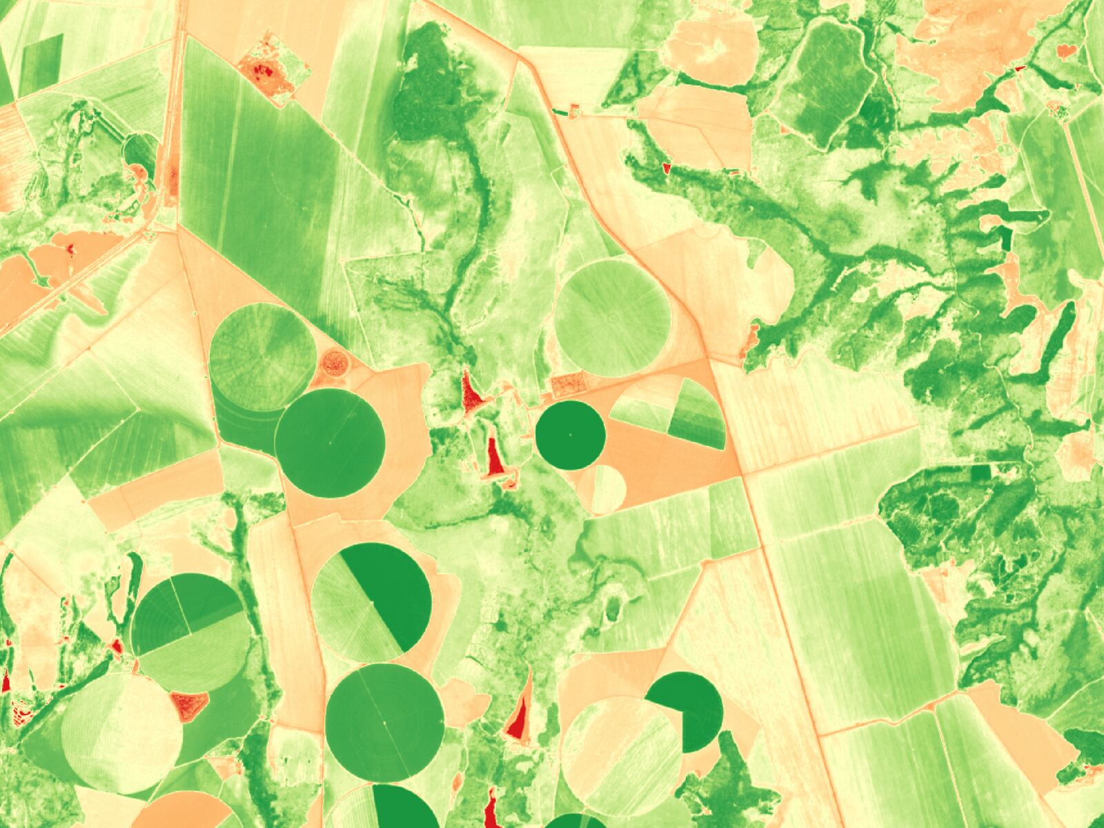
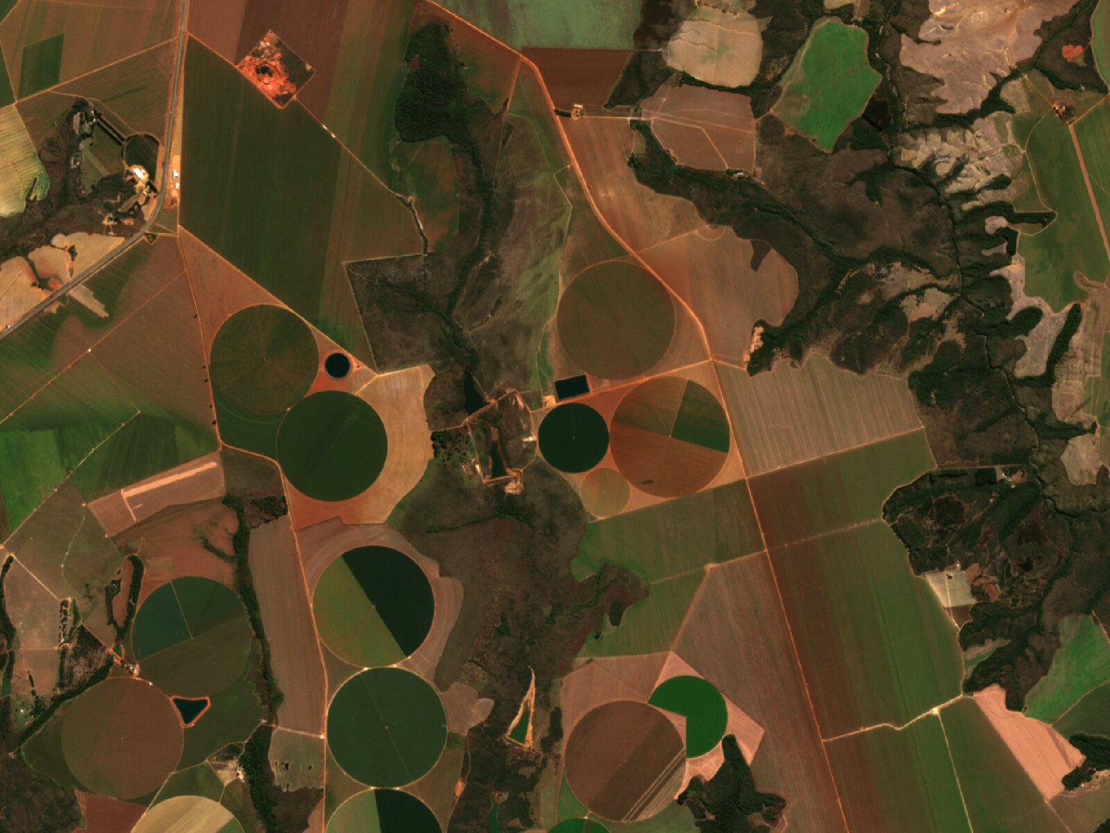
Centre pivots near Cristalina in Sentinel-2 true colour, then the same view as NDVI from red to green (after) — Cristalina, 7 July 2026, 11.4 by 8.6 km. Drag the handle: the circles that look dark in true colour split into growing (deep green) and resting (orange). Contains modified Copernicus Sentinel data 2026.

Centre pivots near Cristalina in Sentinel-2 true colour, then the same view as NDVI from red to green (before) — Cristalina, 7 July 2026, 11.4 by 8.6 km. Drag the handle: the circles that look dark in true colour split into growing (deep green) and resting (orange). Contains modified Copernicus Sentinel data 2026.

To keep a copy, right-click the layer, Export > Save As…, and write a GeoTIFF clipped to your extent. You get the 10 m pixels of your area and nothing else.

Use it when: you want to see a place on a date, build a composite or compute an index, and QGIS is 3.42 or newer.

Skip it when: you work offline, or you need hundreds of scenes for a time series. A script against the same STAC API is the tool for that.

Method 3: The Semi-Automatic Classification Plugin

The Semi-Automatic Classification Plugin (SCP) has a Download products tab, and it still works for Sentinel-2 in 2026. SCP 8.5 is the version for QGIS 3, and the 9.0 series on the plugin repository is for QGIS 4. It is built on the Remotior Sensus library, and the plugin page says it "requires the installation of additional dependencies".

I tested its search engine, Remotior Sensus 0.7.7, on the same area. The "Sentinel-2" source queries the Copernicus catalogue and listed the 7 and 17 July scenes in 26 seconds. Without Copernicus credentials, SCP downloads the product from Google Cloud's public Sentinel-2 bucket, and that bucket holds the 7 July L2A product. The "Sentinel-2_MPC" source asks Planetary Computer and answered in 0.2 seconds.

The part that cost me time was the install. SCP needs Remotior Sensus and SciPy in QGIS's own Python. On the macOS QGIS 3.44.7 app, SciPy installed with pip would not load, so I ran the search outside the plugin. On Windows and Linux, follow the installation chapter of the SCP manual.

Use it when: you are going to classify the image in SCP anyway. It downloads, converts to reflectance and builds the band set in one place.

Skip it when: you only need an image or an index. Method 2 has nothing to install.

Method 4: Ask an AI agent in QGIS

We build one of these tools, AI Agent, a chat panel inside QGIS that runs the steps in the project you have open. This section is about our own tool.

In an empty project, I typed:

Find the least cloudy Sentinel-2 image of the center pivots around Cristalina, Brazil, from July 2026, show it in true colour, then add an NDVI layer.

2:47min

from Send to answer

actions in one message

0.00068%

cloud on the scene it picked

133km²

of 10 m NDVI

It geocoded Cristalina, searched Earth Search for July 2026 and picked the 7 July scene from Sentinel-2C on tile 22KHG, at 0.00068% cloud. That is the lowest of the 18 July scenes over the town, the same answer Methods 1 and 2 gave by hand. It streamed the true colour, red and NIR COGs, asked once before adding them, computed NDVI at 10 m over a 133 km² box around the pivots and styled it from red to green.

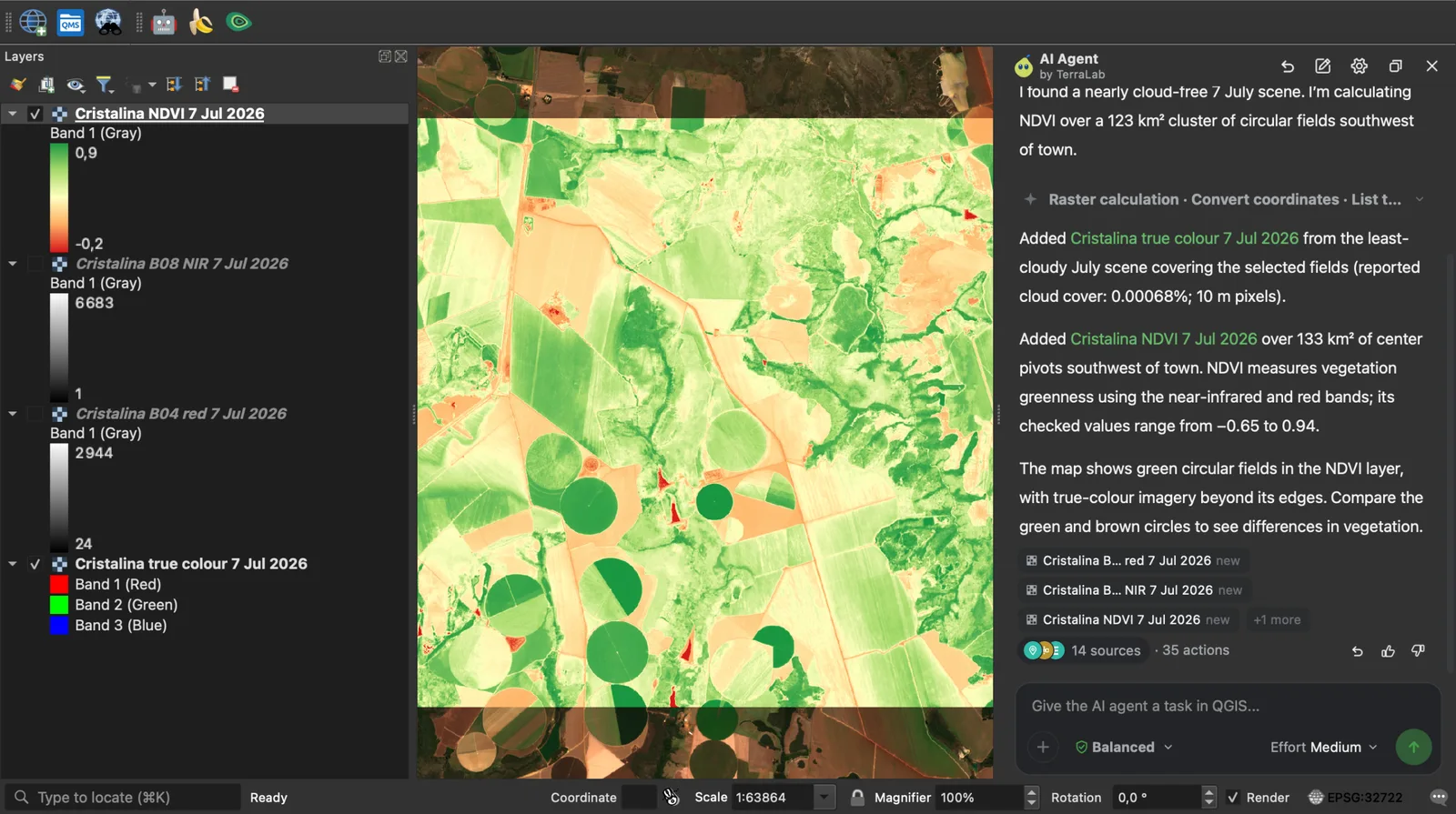
QGIS with the Cristalina NDVI layer from red to green over the true colour image, the Layers panel with the NDVI legend from -0.2 to 0.9, and the AI Agent panel giving the date, the 0.00068% cloud cover and the NDVI range -0.65 to 0.94. — The answer beside the result: the scene date, its cloud cover, the 10 m pixel size and the NDVI range, −0.65 to 0.94.

The NDVI is a GeoTIFF on disk and the imagery stays streamed, as in Method 2. The limit is the extent: it computed NDVI on the box it chose around the pivots, not the whole 110 km tile, so name a bigger area when you need one.

Try AI Agent for free in QGIS

The question users ask right after is what changed. In the same chat I sent:

Now compare it with the least cloudy image of the same area from July 2025 and show which fields gained or lost vegetation.

In 2 minutes 43 seconds it took the 17 July 2025 scene from Sentinel-2B (0.0006% cloud), computed its NDVI on the same 10 m grid and mapped the difference with a 0.10 threshold. Over the 133 km², 39.14 km² gained vegetation and 14.52 km² lost it. It added its own caveat: the two images are ten days apart in the season, so crop stage explains part of the change. Its checkpoint undoes either message in one click.

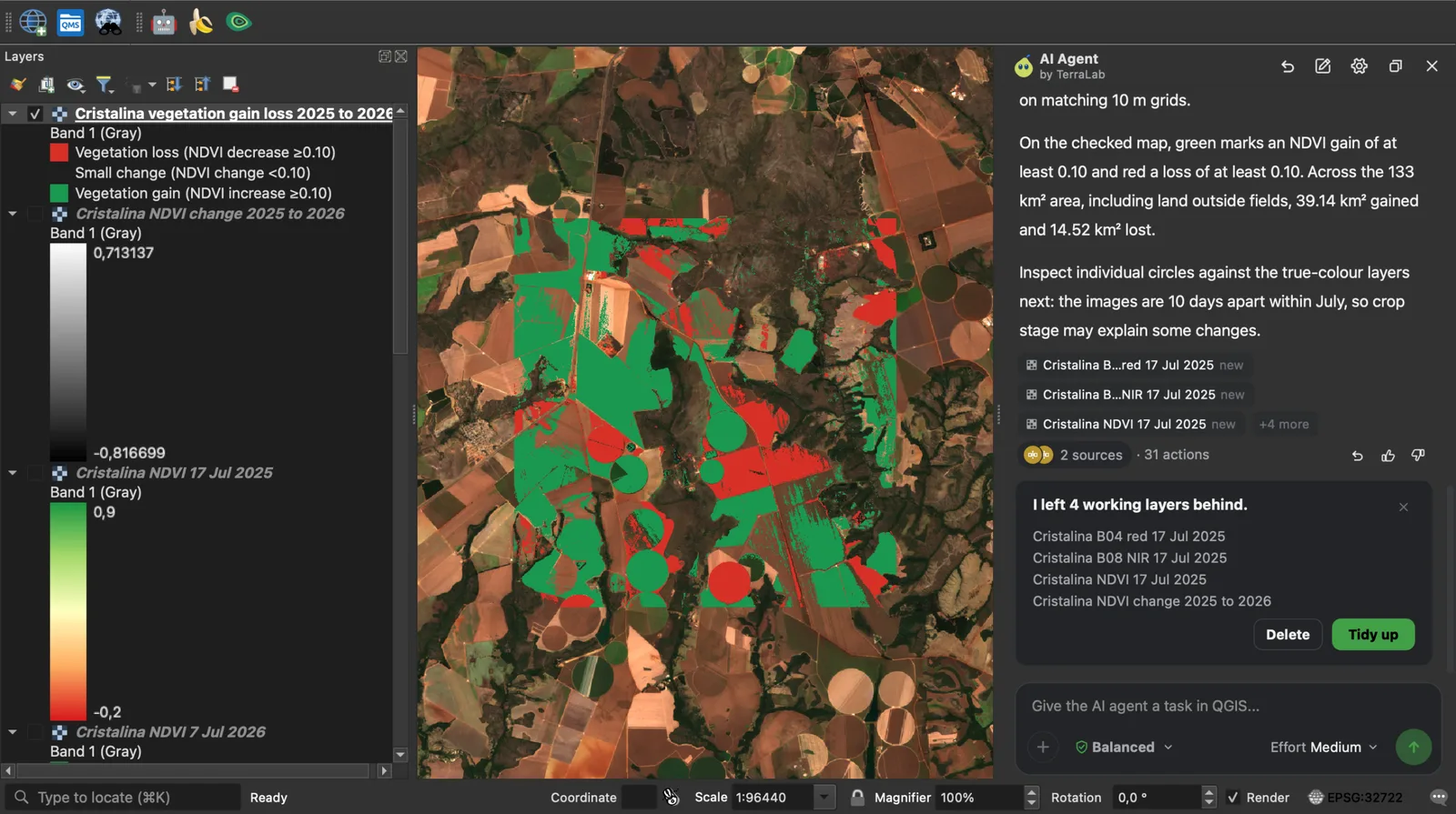
QGIS with pivots and fields coloured green for NDVI gain and red for NDVI loss between July 2025 and July 2026 near Cristalina, and the AI Agent answer giving 39.14 km² gained and 14.52 km² lost. — July 2025 to July 2026: green gained at least 0.10 NDVI, red lost at least 0.10. Whole circles change sign from one year to the next.

Use it when: you want the scene picked, streamed and turned into an index or a comparison in one step, or you don't want to look up band names and offsets.

Skip it when: you need the full product archived offline. That is Method 1. The free plan is 10 messages a month, and these two runs used two.

What to remember

For most work, stream Sentinel-2 over STAC: Layer > Data Source Manager, STAC tab, Earth Search, then right-click a scene, Add Layer. No account and no 1.1 GB download.
Download the L2A .SAFE product from Copernicus Browser, with a free account, when you need every band offline.
True colour is B4, B3, B2 and NDVI is (B8 − B4) / (B8 + B4), both at 10 m, on Level-2A for anything you compare across dates.
Since processing baseline 04.00 (January 2022), raw L2A values carry an offset of 1,000: remove it before NDVI unless your source already did, and check one pixel with Identify first.
A scene's cloud percentage covers its 110 km tile, not your field. The same pass over Cristalina read 22% on one tile and 2.6% on the other.

Questions people ask

Do I need a Copernicus account to get Sentinel-2 images?

Not to stream them. Earth Search over STAC, SCP's Google Cloud route and AI Agent all worked without one. You need a free Copernicus Data Space Ecosystem account to download the product from Copernicus Browser, and for the Sentinel Hub plugin.

L1C or L2A: which one should I download?

L2A for almost everything. It is corrected for the atmosphere, so a field reads the same on a hazy day and a clear one, and it carries the SCL band that flags cloud and shadow. L1C is top-of-atmosphere reflectance, smaller (about 760 MB against 1,090 MB for the same pass over Cristalina), and suits you when you run your own atmospheric correction.

Which Sentinel-2 bands give true colour, and which give NDVI?

True colour is B4 red, B3 green and B2 blue, and every L2A product also ships it ready-made as TCI. NDVI uses B8, the near infrared, and B4: (B8 − B4) / (B8 + B4). All four bands are 10 m. On raw L2A values from processing baseline 04.00 onwards, subtract 1,000 from each band first.

How do I filter Sentinel-2 images by cloud cover?

In Copernicus Browser, the cloud slider under Sentinel-2 in the Search tab. QGIS 3.44's STAC search has no cloud filter, so read the thumbnails, or eo:cloud_cover under Details…. Either way the number covers the whole tile. For the pixels of your field, the L2A SCL band marks cloud shadow as 3 and cloud as 8 and 9.

Can I stream Sentinel-2 into QGIS instead of downloading it?

Yes, from QGIS 3.40 in the Browser panel and from 3.42 with search in the Data Source Manager. The bands are Cloud-Optimized GeoTIFFs, and QGIS reads only the tiles it draws: 5.4 seconds for a 133 km² view at 10 m in my test. Save a clipped copy with Export > Save As… when you need it offline.

Does the Sentinel Hub plugin still work?

It is maintained: version 2.0.8 came out on 9 June 2026 on the QGIS plugin repository. It needs a Copernicus Data Space or Sentinel Hub account plus an OAuth client, and its page warns that the Copernicus endpoint may not work on macOS. Copernicus's own documentation describes it as a viewer and sends single downloads to Copernicus Browser. I did not test it for this post.

For more on what a chat panel can do in QGIS, the AI Agent guide has ten more real runs, and the QGIS AI hub collects the rest. To turn the NDVI above into field polygons, the raster to vector post picks up from here. The two companion tutorials cover downloading OpenStreetMap data and georeferencing a scanned map.