Detect Solar Panels in QGIS: 5 Methods
Published Updated
To map rooftop solar in QGIS, start with what somebody has already mapped. Open Vector > QuickOSM > QuickOSM…, put generator:source in the key box and solar in the value box, run it on your area. OpenStreetMap carries 6,143,024 objects with that tag, read 3 September 2026, so in a well surveyed town you are finished in two minutes. Where coverage is thin you detect the arrays yourself, and the method depends on your bands and your pixel size.
 , start with what somebody has already mapped. Open
 | Your input | Method | What it costs |
|---|---|---|
| An area OpenStreetMap already surveys well | Method 1, QuickOSM | Free |
| Any raster the canvas shows, on any machine | Method 2, a cloud segmentation model | Free 1.5 km² a month, then €39 |
| Multispectral imagery with a near-infrared band | Method 3, Raster > Raster Calculator… | Free, core QGIS |
| Four bands or more, and time to draw training areas | Method 4, Semi-Automatic Classification Plugin | Free plugin |
| An RGB orthophoto near 20 cm, and a GPU or patience | Method 5, Deepness plus its Solar PV model | Free |
Every price, plugin version and tag count here was read on 3 September 2026.
Method 1: Take what is already mapped
QGIS dropped its own OSM downloader in 3.0 and pointed users at QuickOSM, so install that first.
Query the generators
Vector > QuickOSM > QuickOSM…, key generator:source, value solar, run on your extent or a named area. Rooftop arrays carry power=generator and often generator:method=photovoltaic.
Query the plants separately
Ground-mounted farms are tagged power=plant with plant:source=solar, a different query. Miss it and every farm is missing from your layer.
Go to the registry for kilowatts
Germany's Marktstammdatenregister ships daily as XML, but suppresses coordinates for any unit at 30 kW or less, so a rooftop lands on a postcode. France's registry stops at the IRIS zone and folds everything under 36 kW into aggregate rows.

Three open datasets serve as training data or a benchmark. Bradbury et al., 19,863 annotated PV polygons over four Californian cities at 30 cm, CC0. BDAPPV, 28,807 French installations with masks, CC BY 4.0. DeepSolar counted 1.47 million systems across the contiguous United States, but released census-tract counts, not polygons.
Use it when: somebody has surveyed your area, or you need capacity rather than shapes.
Skip it when: the coverage is patchy, which you only find out by looking.
Method 2: A cloud segmentation model
A segmentation model has learned what an array looks like, so it separates one from a dark roof where Methods 3 and 4 cannot. We build one of these, AI Segmentation. This section is about our own tool.
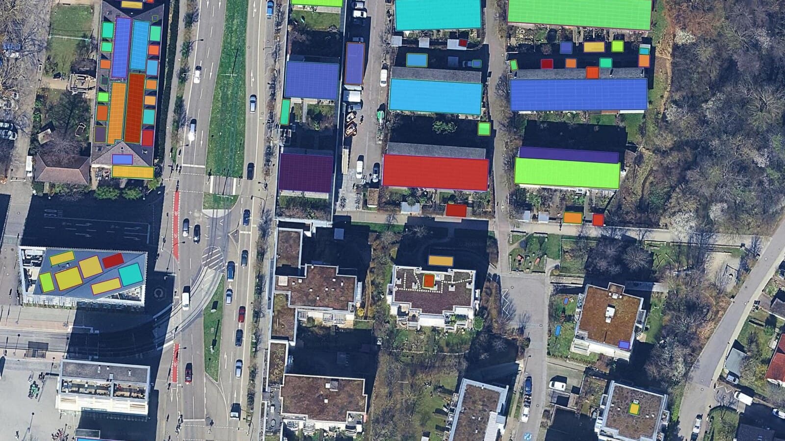
Draw a zone over whatever raster the canvas shows, type solar panel, and each array comes back as a polygon in the project CRS with an area and a confidence score. The model runs on our servers in Europe, so there is no card and no Python environment.

Between 5 July and 1 September 2026, 47 people outside our team ran solar panel 104 times, and 15.6% of tiles came back empty. Across 96 exported runs the model found 40,088 candidates and they kept 14,245, or 35.5%, covering 496,931 m² of panel.
Type solar panel, not solar farm. The second asks for the installation, and the model answers with one uniform surface or nothing. On the few runs we have, it left 21 of 24 tiles empty.
Best for: rooftop arrays across a district, on any machine.
Not for: a module count. A dense array returns as one surface, so split it in QGIS or divide by the module footprint you know. A residential module is roughly 1.7 m by 1.1 m.
Price: free for 1.5 km² a month, no card. Pro is €39 a month excluding VAT. Try Pro free for 7 days: add a card, cancel before the end and nothing is charged.
Runs on: our servers, in Europe.
Install: the plugin manager, QGIS 3.22 or later, then sign in from the panel.
Method 3: Threshold in the raster calculator
Work in a projected CRS, because two steps below take an area in layer units.

Raster > Raster Calculator…, algorithm id native:rastercalc. Panels are dark, and in the near infrared much darker than a dark roof, so a normalised index between the red and NIR bands separates them on most scenes. Then gdal:sieve drops the speckle and gdal:polygonize makes polygons.
On three bands of RGB this fails, because a dark roof and a panel share their values. Texture is the usual rescue. grass:r.texture computes thirteen GLCM measures, and arrays score high on contrast and low on inverse difference moment. GRASS ships with the Windows installer and not with the macOS bundle.
Use it when: you have a near-infrared band and one clean scene.
Skip it when: the imagery is RGB, or the thresholds have to hold across a mosaic shot on different days.
Method 4: Supervised classification with SCP
The Semi-Automatic Classification Plugin adds an SCP menu and an SCP Dock. Build a Band set, draw ROIs over panels and over each lookalike, then classify with Maximum Likelihood, Minimum Distance, Spectral Angle Mapping, Random Forest, Support Vector Machine or a Multi-layer Perceptron. Version 8.5.0 is what QGIS 3.x installs, GPL v3, downloaded 2,644,482 times.
Its own FAQ rules out the input most people have. "You cannot use orthophotos with less than 4 bands", because below four the algorithms cannot separate the classes.
Use it when: you have four bands or more and want a repeatable, documented classification.
Skip it when: your input is an RGB orthophoto or a basemap.
Method 5: A local model in Deepness
Ground resolution decides everything. Bradbury et al. built their reference PV dataset at 30 cm because "solar panels are typically between 1 and 2 meters in length", which puts several pixels on each one. That resolves the array, not the modules inside it. Clark and Pacifici found individual panels "difficult to distinguish even at 15.5 cm resolution". Published rooftop PV work sits between 10 cm and 31 cm. Sentinel-2 at 10 m is for farms, never roofs.
Deepness runs ONNX models inside QGIS, free and Apache 2.0, and its model zoo ships a Solar PV Segmentation model at 20 cm/px trained by Kleebauer et al. and hosted by Fraunhofer. Point it at your orthophoto and you get a panel mask, no account, nothing leaving your machine.
Speed is the catch. A user measured that same model at "80+ minutes for a digital Orthophoto tile (20 cm resultion, 5000 points in each direction)" on a CPU, and the issue is still open. Beyond this one there is no well maintained open rooftop PV model.
Use it when: nothing may leave the machine, and your ortho is near 20 cm.
Skip it when: you have no NVIDIA card and a district to cover.
The five methods side by side
| QuickOSM | AI Segmentation | Raster calculator | SCP | Deepness | |
|---|---|---|---|---|---|
| Bands needed | None | Three | NIR helps | Four or more | Three |
| Imagery stays local | Yes | No | Yes | Yes | Yes |
| GPU | No | No | No | No | Recommended |
| Output | OSM polygons | Polygon per array | Raster mask | Class raster | Panel mask |
| Cost | Free | Free tier, then €39 | Free | Free | Free |
What to remember
Query OpenStreetMap before anything else, because a surveyed town is finished in two minutes and no detection beats a mapper who has been there.
If the imagery may not leave the machine, Deepness and its local Solar PV model keep everything on your machine.
On an RGB basemap the raster calculator and SCP are out, because neither separates a panel from a dark roof by value alone.
Around 30 cm resolves an array and nothing resolves the modules inside it, so map areas and never count panels from imagery.
Kilowatts come from a utility registry, never from a picture, and both the French and the German registry blur the location of small rooftop units.
Try it free in QGIS, no card needed
Questions people ask
Can QGIS detect solar panels on its own?
No. Core QGIS has thresholding and polygonizing, which need a spectral difference, so an RGB basemap gives you nothing. Detection comes from a plugin, Deepness locally or ours in the cloud.
What imagery resolution do I need?
Around 30 cm resolves an array, following Bradbury et al. Individual modules are hard even at 15.5 cm, so plan on mapping arrays and areas rather than counting panels.
How do I tell a solar panel from a dark roof?
You cannot, on three bands, by value alone. Use a near-infrared band, a texture measure like grass:r.texture, or a model that has learned what an array looks like.
Does it find ground-mounted solar farms too?
Yes, and in OpenStreetMap they are a separate query, power=plant with plant:source=solar. With a model, type solar panel for the farm too, because it detects each panel rather than the site.
Can I count how many panels are installed?
Not from imagery. Detection gives outlines and surface area. The module count and the kilowatts come from a registry, and in France that stops at the IRIS zone.
The building footprints guide walks the filtering step in full, and the SAM in QGIS post covers which objects these models find well. For running the detection and the area count together as one instruction instead of stepping through the plugin by hand, AI Agent does that inside the same QGIS project. The QGIS AI hub compares the plugins, and the product page is AI Segmentation.