Extract Roads in QGIS: 6 Methods, OSM Checked in 4 Towns
Published Updated
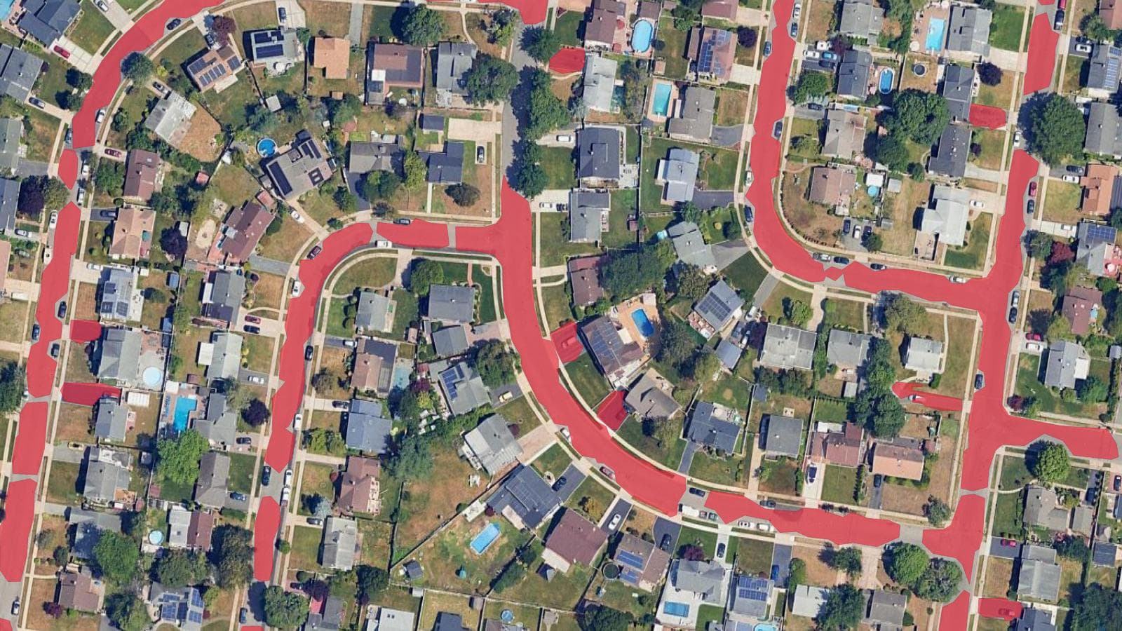
To extract roads in QGIS, install QuickOSM, open Vector > QuickOSM > QuickOSM, query the key highway over your canvas extent, and the network arrives as lines in seconds. Where OpenStreetMap is thin, five other methods put roads on the map: a segmentation model, a published national dataset, hand digitizing, GRASS thinning, and supervised classification.
 , install QuickOSM, open
 One choice comes first, and it decides which methods are open to you. You are not extracting roads. You are choosing between a centreline, one line down the middle carrying lane count and speed limit, and a surface, the tarmac kerb to kerb. Routing needs the line. Drainage and resurfacing quantities need the area. Half the methods below give you one, half give you the other, and converting between them costs an extra step.
| What you are working with | Method | What it costs |
|---|---|---|
| A city with active OSM mappers | 1, QuickOSM | Free |
| Recent imagery of somewhere OSM has not reached | 2, a segmentation model | Free tiers, then a subscription |
| A country with a national road dataset | 3, download and clip | Free |
| A handful of roads, or fixes to a layer you hold | 4, digitize with tracing on | Free, and slow |
| A road mask or a scanned map | 5, GRASS r.thin then r.to.vect | Free |
| A multiband scene where tarmac stands out | 6, supervised classification | Free plugin, hours of samples |
Every price, version and menu path here was read on 3 September 2026, against the QGIS 3.44 manual and each tool's own documentation.
Method 1: Roads from OpenStreetMap with QuickOSM
Thirty seconds of checking OSM saves you every method below. QuickOSM queries the Overpass API and drops the answer straight into your project.
Install QuickOSM
Plugins > Manage and Install Plugins, search QuickOSM, install.
Open the quick query
Vector > QuickOSM > QuickOSM, Quick query tab.
Set the key
Key highway, value empty for every road class. Add a value to narrow it: residential, track, motorway.
Bound it
Pick Canvas Extent. An unbounded country query times out on Overpass.
Run and filter
Lines arrive with the OSM tags attached. Filter on highway, and read surface where it exists.

The tags are the reason a mapped area beats any detection. highway=track tells you a way is an agricultural track and highway=unclassified that it is a minor public road. No model on this page can tell you either one, because a detection returns a shape and OSM returns a shape somebody has already named. Attribution is required under the ODbL.
Coverage is where OSM stops. Open the highway lines over recent imagery in rural Africa, in South Asia, or on the growing edge of most cities, and the tracks sit plainly in the picture with nothing drawn on them.

Use it when: somebody has already mapped the area.
Skip it when: the imagery shows roads the OSM layer does not.
How complete is OpenStreetMap? Four French communes, measured
In four French communes we measured on 23 September 2026, OpenStreetMap held 96 to 98% of the paved road length in IGN's official BD TOPO, while 20 to 32% of IGN's farm and forest tracks were absent from it in the three rural ones, and Microsoft's free detections found 6 to 12% of those missing tracks. In a country mapped as well as France, extracting roads from imagery is a track problem, not a road problem.
| Commune | IGN paved roads | Absent from OSM | IGN tracks | Absent from OSM | Of those, Microsoft found |
|---|---|---|---|---|---|
| Villeurbanne, dense city, 15 km2 | 280 km | 10.3 km (3.7%) | 15 km | 0.8 km (6%) | 0.3 km |
| Orgères-en-Beauce, open farmland, 15 km2 | 27 km | 0.5 km (2.0%) | 27 km | 5.6 km (21%) | 0.7 km (12%) |
| Saint-Léonard-de-Noblat, hedged farmland, 55 km2 | 147 km | 3.9 km (2.6%) | 113 km | 36.4 km (32%) | 2.2 km (6%) |
| Gérardmer, mountain forest, 56 km2 | 216 km | 3.8 km (1.7%) | 228 km | 44.7 km (20%) | 2.8 km (6%) |
In these four communes, Microsoft's lines cover 89 to 95% of IGN's paved road length and 17 to 37% of its tracks.
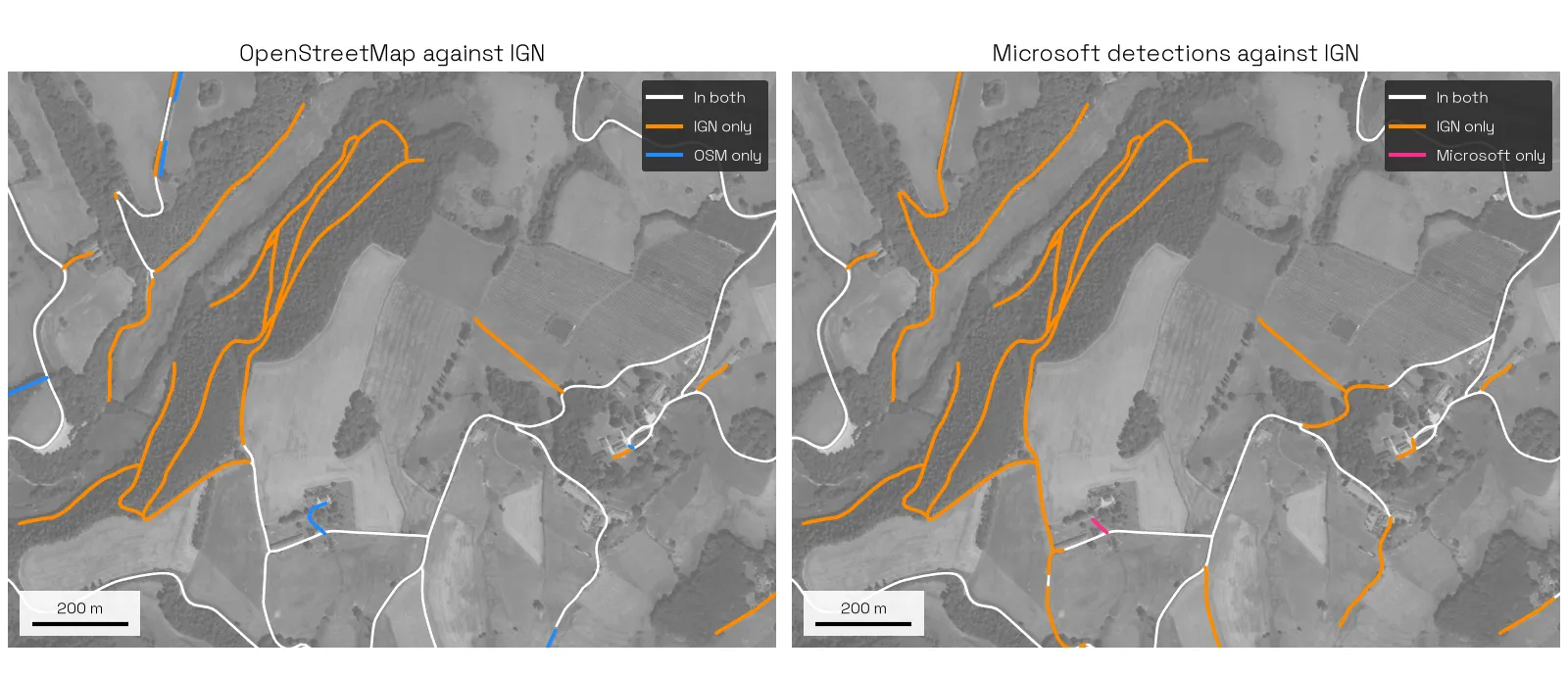
Where the missing tracks lie decides whether imagery can find them. We drew 20 missing pieces at random in each rural commune and looked at each one on IGN's orthophoto. In Orgères-en-Beauce, 7 show a track on the ground and 5 fall on a bare field edge with nothing to trace. In Gérardmer, 15 of 20 run under conifer canopy, where no model looking down will ever see them. Saint-Léonard sits between the two, with 7 visible and 5 under trees.
Two more things turned up that change how you query. In Gérardmer, another 93 km of IGN's tracks sit in OSM as highway=path, so a QuickOSM query for track alone misses them: leave the value empty. And OSM holds what IGN does not draw, such as 100 km of footpaths and trails in Gérardmer and 64 km of service roads in Villeurbanne (car park aisles, yards, driveways).
How we measured this
We took IGN BD TOPO troncon_de_route from the Géoplateforme WFS, every OSM highway way from Overpass on 22 and 23 September 2026 (what QuickOSM returns, sidewalks set aside), and Microsoft's 28 April 2025 drop, clipped to each commune. Every line was cut into 10 m pieces, and a piece counts as absent when the other dataset has no line within 10 m running within 45 degrees of it. At 5 m or 20 m, paved roads stay under 5% absent and rural tracks between 15 and 37%. Four communes are not France, BD TOPO is a reference rather than the truth (5 of the 20 Orgères pieces showed nothing on the ground), and the orthophoto check is one reader's call on 60 images.
Method 2: A segmentation model
A segmentation model has learned what a road looks like, so shape and context carry it past the look-alikes that stop Method 6. We build one of these, AI Segmentation (complete guide). This section is about our own tool.
Install from the plugin manager
QGIS 3.22 or later on Windows, macOS or Linux. No GPU, no Python environment, no weights to fetch.
Draw the area
Over whatever raster the canvas already shows, from a satellite scene to a WMS.
Type the word
road for the carriageway. parking lot, sidewalk and driveway are separate words. Run them separately, or a car park pressed against a road merges into it.
Filter, then convert if you need lines
Once the run has returned the polygons, they carry label, class, score, area_m2 and perimeter_m in the project CRS. Filter on score and area, then send the surface through GRASS v.voronoi.skeleton for a centreline.

Output is polygons kerb to kerb and never centrelines, so a line deliverable costs you the skeleton step above. Both cloud modes send imagery to a server in the European Union, and only the small local model stays on your machine.
Tree canopy breaks the surface into pieces you rejoin by hand, and bridge decks do the same. Wet asphalt and fresh resurfacing change the tone enough to drop a stretch. We publish no accuracy figure, because the number moves with your imagery.

One number from our own tuning table, because it explains a result people find strange. Roads run on a coarser tile than buildings, floored at 512 m of ground per tile against 128 m for a building, because a model handed a fragment of tarmac calls it a car park. A road only reads as a road when the model can see a run of it.
Costs, read 28 September 2026. The free plan covers 1.5 km2 of ground a month on Automatic with no card, plus 20 object detections a month on cloud Semi-Auto, and Semi-Auto on your own machine has no counter at all. Pro raises those to 100 km2 and 500 objects for €39 a month excluding VAT. Mapflow ships a roads model priced in credits at 0.10 dollars each, 5 credits per km2 plus the imagery cost, with 250 credits free to start.
Use it when: the imagery is newer than the map, and there is more road than you would draw by hand.
Skip it when: OSM already holds the network, or the imagery cannot leave your machine.
Try it free in QGIS, no card needed
Method 3: Published road datasets
Somebody may have run the detection already and given the result away.
Microsoft Road Detections covers 54.2 million kilometres of road across 235 countries, mined from Bing Maps aerial imagery and released under the ODbL as centrelines, one file per world region. In the four French communes measured above, it held about nine in ten kilometres of paved road and one in five of track.
Meta publishes its own AI-generated roads through the Rapid editor. The Daylight distribution that used to package them was sunset in May 2024, so Rapid is now the practical route to them.
National agencies beat both where they exist. France publishes BD TOPO with its Troncons de route layer at metric precision under Etalab 2.0, against the rough alignment a mined dataset gives you. Great Britain publishes OS Open Roads free through the OS Data Hub, refreshed each April and October.
The catch is vintage. A detection set is a snapshot of the imagery it was mined from, and none of these knows that a road closed last spring.
Use it when: you need national coverage this afternoon and the date is good enough.
Skip it when: the job is a change since the dataset was built.
Method 4: Digitize by hand, with tracing on
Under about fifty roads, drawing them still wins, and QGIS gives you real help once you know what tracing actually follows.
Toggle editing, pick Add Line Feature, then enable the Tracing tool on the Snapping toolbar or press T. Snap to a vertex, move to a second one, and QGIS builds the shortest path between them along existing feature edges. Unfold the tracing icon and set Offset to digitize parallel to those features rather than along them.
Two behaviours surprise people. Tracing switches itself off when the canvas holds too many features, and comes back when you zoom in. For a freehand curve, R gives you streaming digitizing instead.
Use it when: under about fifty roads, or corrections against a layer you already trust.
Skip it when: you are staring at a district of unmapped tracks.
Method 5: GRASS r.thin, then r.to.vect
Work in a projected CRS. Two steps below take a width in layer units, and a width in degrees is meaningless.
This is the one method that hands you centrelines directly, which is why it survives in 2026. Feed it a raster where road is one value and everything else is another: a thresholded scan of a paper map, or a mask from Method 2 or 6.
r.thin reduces every stroke to one pixel wide, and that pixel chain is the centreline. r.to.vect with feature type line turns it into geometry. The GRASS manual warns that it creates excessive nodes at junctions and dangling spurs, so budget the cleanup: drop the spurs by length, then merge the segments that should be one road.
GRASS ships with most QGIS installers, so there is nothing extra to buy. It is also the step that turns a Method 2 surface into a line network, which is the pairing I use most.
Use it when: you hold a clean road mask or a clean scan, and you need lines.
Skip it when: the input is a colour photograph.
Method 6: Supervised classification
Classify the pixels, then vectorize the road class. The Semi-Automatic Classification Plugin is the standard tool, by Luca Congedo. Release 9.0.4 needs QGIS 3.99, the QGIS 4 line, so on QGIS 3.x the manager serves you 8.5.0 instead. dzetsaka does the same job with a smaller interface.
You draw training regions on road pixels and on every other class in the scene, run a classifier such as Maximum Likelihood, then send the road class through Raster > Conversion > Polygonize. The raster to vector guide covers that second half, including the algorithms that fix the staircase edges polygonize leaves behind.
It works when tarmac genuinely differs from what surrounds it, and multispectral bands help. It falls over on the look-alikes, because a classifier compares pixel values and knows nothing about shape: grey roofs, dry riverbeds and bare field margins all land in the road class. Budget hours for the training samples, and expect to redraw them for the next scene.
Use it when: you have multispectral bands and roads that stand out in them.
Skip it when: roads and roofs share a colour, which is most cities.
What to remember
Four things break every method on this page, whatever you paid for it. Tree canopy over a residential street hides the road from any sensor looking down, so the result comes back in pieces. A dirt track and the field beside it are the same colour, which is why unpaved roads go missing in exactly the places that need them mapped.
The other two are shape problems. Rivers, dry riverbeds and railway lines are long thin features, and any pixel-based method drops them into the road class. Bridges and tunnel mouths cut the surface at the point where a network most needs to stay joined.
Check OpenStreetMap first, because thirty seconds there decides whether the other five methods are worth opening. In a well-mapped country, what is left to find is mostly tracks, and much of that sits under trees.
A Method 2 surface run through Method 5 gives you a centreline network that nobody had to digitize.
Try it free in QGIS, no card needed
Questions people ask
Can QGIS extract roads from satellite imagery on its own?
Not automatically. Core QGIS digitizes by hand and vectorizes rasters you have already classified. Getting roads out of a photograph needs a plugin: a segmentation model, or a classifier such as SCP that you train yourself.
Does road extraction give lines or polygons?
Both exist, and the method decides. OSM, national datasets, published detections and GRASS r.thin return lines. Supervised classification and segmentation models return surfaces, because a surface is what the imagery shows. GRASS v.voronoi.skeleton converts one to the other.
Why do roads under tree cover come out broken?
No sensor looking down sees through a canopy, so the gap is in the data before any software touches it. Bridge the pieces by snapping the segments together in an editing session.
How complete is OpenStreetMap's road network?
For paved roads in a well-mapped country, close to complete: OSM held 96 to 98% of IGN's paved road length in the four French communes we measured in September 2026. Tracks are the gap, with 20 to 32% of IGN's track length missing in the rural ones. Worldwide, a 2017 study put OSM's road network at about 83% complete.
Can any method find unpaved tracks?
Partly. A dirt track and the field beside it share a colour, so classification usually misses them and detection models find the wider ones. OSM highway=track is the most reliable source where a mapper has been, which is the problem in the places that need them most.
What imagery resolution is enough for road extraction?
Whatever separates the road from what sits beside it. A motorway shows up in a coarse satellite scene; a residential lane under trees needs 20 cm orthophoto or better. Test your own imagery on a free tier before committing to a method.
Is road extraction free in QGIS?
Methods 1 and 3 to 6 are free to install and free to run. Only the cloud segmentation models charge, and both named here have a free allowance.
Can I turn on tracing and follow a road on the imagery?
Tracing does not look at the picture. The QGIS 3.44 manual is explicit: it builds the shortest path along the edges of existing vector features. Over bare satellite imagery there is nothing to follow, so the tool does nothing at all. It pays off when you already hold parcels or a partial network and want the new geometry to snap to them.
Can I run GRASS r.thin on an aerial photo?
r.thin needs a raster where road is one value and everything else is another. Hand it a colour photograph and it thins whatever the pixel values happen to group into, which is not roads. It is a brilliant tool placed one step too early: it belongs after a classification or a detection, not before.
The raster to vector guide covers the polygonize half of Method 6, and the building footprints guide walks the filtering step end to end. If Method 2's detect-then-skeletonize chain gets repetitive across tiles, AI Agent can run those same steps from a single instruction in QGIS. The QGIS AI hub compares the plugins side by side.