Choropleth Map: Definition, Classification Methods, Examples
Published
A choropleth map is a thematic map that shades predefined areas, such as countries, states, counties or French départements, according to the value of one statistic in each area. Most classed choropleth maps group the values into 5 to 7 colour classes, moving from light to dark as the number grows, and map a rate or density rather than a raw total.
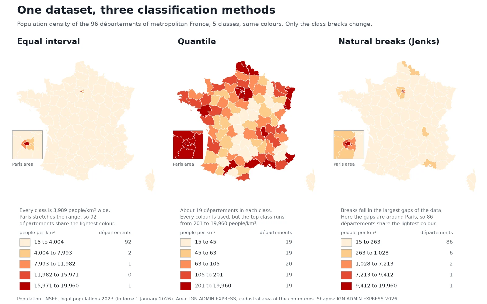
Change the rule that splits the numbers into classes and the same dataset tells a different story. Below, we map the population density of the 96 départements of metropolitan France three ways with the exact same five colours. On the first map, France looks almost empty outside Paris. On the second, two départements in five turn red.
5 to 7classes
usual range on a classed choropleth
ColorBrewer sequential schemes stop at 9
1,350×density gap
Paris vs Lozère in our test dataset
19,960 vs 14.8 people per km²
1826first map
Charles Dupin's schooling map of France
Term coined by J. K. Wright in 1938
What is a choropleth map?
The word comes from the Greek choros (area or region) and plethos (multitude). A choropleth starts with boundaries that already exist, such as census tracts, municipalities or provinces, attaches one number to each polygon, and fills the polygon with the shade that matches its number.
French engineer and mathematician Charles Dupin made the first known choropleth map and presented it on 30 November 1826 (Polish Cartographical Review). His Carte figurative de l'instruction populaire de la France shaded each French département by the number of inhabitants per boy enrolled in school, using darker ink where fewer boys went to school. The name itself came a century later: American geographer John Kirtland Wright introduced the term "choropleth map" in 1938.
A choropleth makes one big assumption: it paints each polygon with a single flat colour, as if the value were uniform from one border to the other. Where the boundaries are cut also changes the picture. Aggregate the same measurements by commune, by département or on a square grid and you get three different patterns, a trap geographers call the modifiable areal unit problem (MAUP).
Why a choropleth map uses rates, not raw counts
A choropleth should map a ratio that does not depend on the area of the polygon: a density (people per km²), a rate (cases per 100,000 residents), a percentage or a per-capita figure (income per person, kWh per household).
When you shade polygons by a raw count, large polygons dominate the map because they cover more ground and collect more of everything. Smaller urban units disappear, even when that is where most of the people or events are concentrated.
Our French dataset shows how wide the gap between count and density gets. We joined the INSEE 2023 legal populations (in force on 1 January 2026, a total of 66,165,815 people across metropolitan France) to the 96 départements from IGN ADMIN EXPRESS 2026, using the sum of the communes' cadastral area for each département:
| Département | Population | Area (km²) | Density (people per km²) |
|---|---|---|---|
| Lozère | 76,486 | 5,167 | 14.8 |
| Creuse | 115,527 | 5,565 | 20.8 |
| Alpes-de-Haute-Provence | 168,054 | 6,926 | 24.3 |
| Val-de-Marne | 1,426,929 | 245 | 5,827 |
| Seine-Saint-Denis | 1,704,316 | 236 | 7,213 |
| Hauts-de-Seine | 1,654,712 | 176 | 9,412 |
| Paris | 2,103,778 | 105 | 19,960 |
Paris packs 2,103,778 people into 105 km², or 19,960 people per km². Lozère spreads 76,486 people across 5,167 km², or 14.8 people per km². Paris is 1,350 times denser, on a polygon 49 times smaller. On a density map, Paris and its three neighbouring départements stand out. On a map of raw totals, a large département reads as important just because it covers more ground.
When the raw total is what your reader needs to see, such as total voters, total sales or total cases, keep the counts and switch map types: place a proportional circle on each area instead of shading the polygon.
Classification methods: equal interval, quantile and natural breaks (Jenks)
Across the 96 départements of metropolitan France, the median population density is 83.5 people per km², while the mean is 568. Paris and its three neighbours pull the mean to nearly seven times the median. On skewed data like this, how you cut the numbers into classes decides what the map shows.
Here is what the three standard classification methods do on our 96 départements when asked for 5 classes:
| Method | How it sets the breaks | Our breaks (people per km²) | Départements per class | Good for | Watch out |
|---|---|---|---|---|---|
| Equal interval | Splits the full range (minimum to maximum) into classes of equal width | 4,004 / 7,993 / 11,982 / 15,971 | 92, 2, 1, 0, 1 | Evenly spread data, temperature or percentages that people read as round steps | One outlier (Paris at 19,960) squeezes 92 of 96 areas into the lightest class, and leaves the 4th class completely empty |
| Quantile (equal count) | Puts the same number of polygons into each class | 45 / 63 / 105 / 201 | 19, 19, 20, 19, 19 | Ranking areas into fifths or quarters, using every colour in the palette | Very different values share a colour (the top class runs from 201 to 19,960), while two nearly identical départements on either side of 63 get different colours |
| Natural breaks (Jenks) | Places breaks in the largest gaps in the data, minimising variance within each class | 263 / 1,028 / 7,213 / 9,412 | 86, 6, 2, 1, 1 | Data with real clusters and jumps | Breaks are tailored to this one table, so you cannot compare two maps made with Jenks; skewed data still piles 86 areas into the bottom class |
George Jenks published the natural breaks method in 1967, building on Walter Fisher's 1958 exact clustering algorithm. Our figure uses the exact Fisher-Jenks optimisation.
QGIS includes four more graduated classification modes (QGIS 3.44 User Manual) that solve specific cases:
 includes four more graduated classification modes (
- Logarithmic scale makes narrow classes for low values and wide classes for high values. When a dataset spans more than three orders of magnitude, like 14.8 to 19,960 people per km², a logarithmic scale separates rural and medium-density départements without letting Paris crush the rest of the legend.
- Pretty Breaks picks clean round numbers (multiples of 1, 2 or 5 times a power of 10) close to the number of classes you asked for, so the legend is easy to read without hand-editing.
- Fixed Interval lets you type the exact step width yourself, for example every 10 percentage points, which is the cleanest way to compare a series of maps across several years.
- Standard Deviation cuts classes by their distance from the mean (such as ±0.5, ±1 and ±2 standard deviations) and pairs well with a diverging colour ramp.
You can also skip classes altogether. An unclassed choropleth maps every value directly onto a continuous colour ramp, so 80 and 180 never fall into the same bucket. The trade-off is that the human eye struggles to match a specific shade on the map back to an exact number on a continuous legend bar.
How many classes and which colours to pick
Most classed choropleth maps use 5 to 7 classes. Use 3 or 4 classes on a small map or dashboard where the reader only needs "low, medium, high". Go up to 7 when the map is large and the values spread smoothly.
Going higher rarely helps. In their 2003 paper introducing ColorBrewer, Mark Harrower and Cynthia Brewer provide schemes from 3 to 12 classes, and note that many sequential schemes stop at 9 classes "because further divisions within the scheme are perceptually unreliable".
ColorBrewer organises its 35 scheme sets into three families, each meant for one kind of data:
- Sequential ramps run from light to dark in one hue or a smooth blend of two (such as the 5-class orange-to-red
OrRdramp in our figure). In print and on bright backgrounds, the cartographic convention is that darker means more. Use a sequential ramp whenever values go from low to high with no natural middle: densities, rates, ages or incomes. - Diverging ramps place a light neutral shade in the middle and step outward into two distinct hues (such as brown to teal, or blue to red). Use a diverging ramp only when the middle class sits on a number that means something in the real world: zero population change, 50% in a two-way vote, or the national average.
- Qualitative palettes use distinct hues of similar brightness with no implied order. They belong on categorical maps (dominant land cover, winning party, zoning type), not on a numeric choropleth.
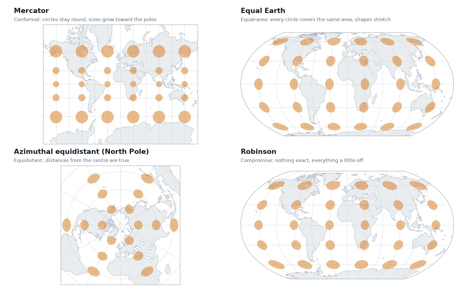
Projection matters alongside colour. Because a choropleth fills the entire area of every polygon with ink, a projection that inflates high latitudes gives northern regions far more visual weight than their true size warrants. Always put a regional or world choropleth in an equal-area map projection, never in Web Mercator. The level of boundary detail should also match your map scale, so tiny coastal islands or slivers do not turn into dark outlines where the fill colour cannot be seen.
Choropleth map vs heat map vs proportional symbols
People often say "heat map" when they mean a choropleth. In GIS, the two take different inputs and answer different questions.
| Map type | Input data | What it draws | Best used for |
|---|---|---|---|
| Choropleth map | Polygons with one value per area | Each region shaded by a rate, density or percentage | Comparing rates across existing administrative boundaries |
| Heat map (kernel density) | Points | A continuous smooth raster surface of point density that ignores borders | Finding where discrete events cluster (road crashes, calls, wildlife sightings) |
| Proportional symbols | Polygons or points with a count | A circle or square on each feature, sized in proportion to the total | Comparing raw totals: population, revenue, case counts |
| Dot density map | Polygons with counts | One dot per N units scattered inside each polygon | Showing how a total is distributed across space without losing the sense of density |
Outside GIS, spreadsheet and analytics tools use "heat map" loosely for any table or grid coloured by value. Inside GIS software, a heat map builds a continuous density surface around point locations; our guide to heat maps in QGIS builds one three ways, from the Heatmap renderer to a kernel density raster. If you start with individual point events and want a choropleth instead, first count the points inside each polygon using a spatial join in QGIS, then divide that count by the polygon's area or population.
How to make a choropleth map in QGIS
Making a choropleth in QGIS takes five steps: load the boundaries, join the table, calculate the rate, set a graduated style and clean up the legend.
Load the polygons and the data table
Drag your boundary layer (such as the départements from IGN ADMIN EXPRESS) into QGIS, then add your statistics table (a CSV or spreadsheet with the official area code and the population or count column).
Join the table to the polygons
Open Layer Properties > Joins on the polygon layer, click the green
+button, and match the shared administrative code in both layers (for exampleINSEE_DEP). If you want a permanent new file instead of an on-the-fly join, run Vector general > Join attributes by field value from the Processing Toolbox.Compute the rate or density
Open the QGIS field calculator, create a decimal field (
real), and divide your count by the denominator. For population density in people per km², use the expression"population" / ($area / 1000000). Make sure your project has a valid ellipsoid set in Project Properties > General so$areareturns square metres on the ellipsoid.Apply a Graduated symbology
Go to Layer Properties > Symbology, switch the renderer at the top from Single Symbol to Graduated, and select your new density field as the Value. Pick a ColorBrewer ramp under Color ramp, choose your Mode (Equal Count (Quantile), Equal Interval, Natural Breaks (Jenks), Pretty Breaks, Standard Deviation, Logarithmic scale or Fixed Interval), set the number of classes (usually 5), and click Classify. Switch to the Histogram tab and click Load Values to see where your break lines sit against the actual distribution of the data.
Round the legend labels and add the source
Double-click the Legend column in the symbol list to round awkward decimals (such as
263.14 - 1028.47to260 to 1,030), state the unit (people per km²) in the legend title, and note the data source and year in your print layout.
If you do not want to hunt down the boundary files and join codes by hand, AI Agent, the QGIS plugin we build, makes a choropleth map from one sentence: it fetches the boundaries and the table, runs the join, calculates the rate and applies the graduated style in your project. For a full worked example with a print layout, see how to make a map in QGIS, which maps the population density of the Paris arrondissements.
Questions people ask
A choropleth map is a thematic map that shades predefined regions, such as countries, states, counties or municipalities, in proportion to a statistical value for each region. It usually groups values into 5 to 7 colour classes along a light-to-dark ramp and maps a rate, density or percentage rather than a raw count.
A choropleth map shades existing administrative polygons (like counties or départements) with one flat colour per polygon based on an aggregated rate or density. A GIS heat map takes point locations and computes a smooth, continuous raster surface of point density that ignores political borders. If your data comes attached to regions, use a choropleth; if your data is a cloud of individual coordinates, use a heat map.
Mapping raw totals on a choropleth makes geographically large regions look more important because they cover more land and contain more people or events. Normalising the count into a density (per km²), a per-capita figure or a percentage removes the distortion of polygon size. When you need to show raw totals by area, place proportional circles on the polygons instead of shading them.
There is no single best method because the right choice depends on how your numbers are distributed. Use Equal Interval or Pretty Breaks when the data is evenly spread from minimum to maximum, Quantile when you want to rank regions into equal-sized groups (such as top fifth and bottom fifth), and Natural Breaks (Jenks) or a Logarithmic scale when the data is skewed with outliers. Always check the histogram in your GIS software before publishing: on our 96 French départements, Equal Interval puts 92 areas into a single colour, while Quantile spreads them evenly across all five.
Five to seven classes work best for most choropleth maps. Fewer than four hides geographic variation, while more than seven makes neighbouring shades on a sequential colour ramp hard for the human eye to tell apart across the map. ColorBrewer caps many of its sequential palettes at 9 classes because finer splits become perceptually unreliable.
In QGIS, join your statistics table to your polygon layer under Layer Properties > Joins, then compute your rate or density in the Field Calculator (for example "population" / ($area / 1000000)). Open Layer Properties > Symbology, change the renderer to Graduated, pick your rate column, select a ColorBrewer colour ramp and a classification mode such as Quantile or Natural Breaks (Jenks), set the class count to 5, and click Classify.
Do it in QGIS by asking for it
AI Agent carries out the task you describe, in your own QGIS project. Free, no card.