QGIS Tutorial for Beginners: First Map in 30 Minutes
Published
To learn QGIS, build one real map from start to finish. This tutorial takes an empty QGIS window to an exported map in seven steps: tour the window, add a basemap, load data, style it, read its table, run one analysis and print the result. Plan about 30 minutes.
 , build one real map from start to finish. This tutorial takes an empty QGIS window to an exported map in seven steps: tour the window, add a basemap, load data, style it, read its table, run one analysis and print the result. Plan about 30 minutes.
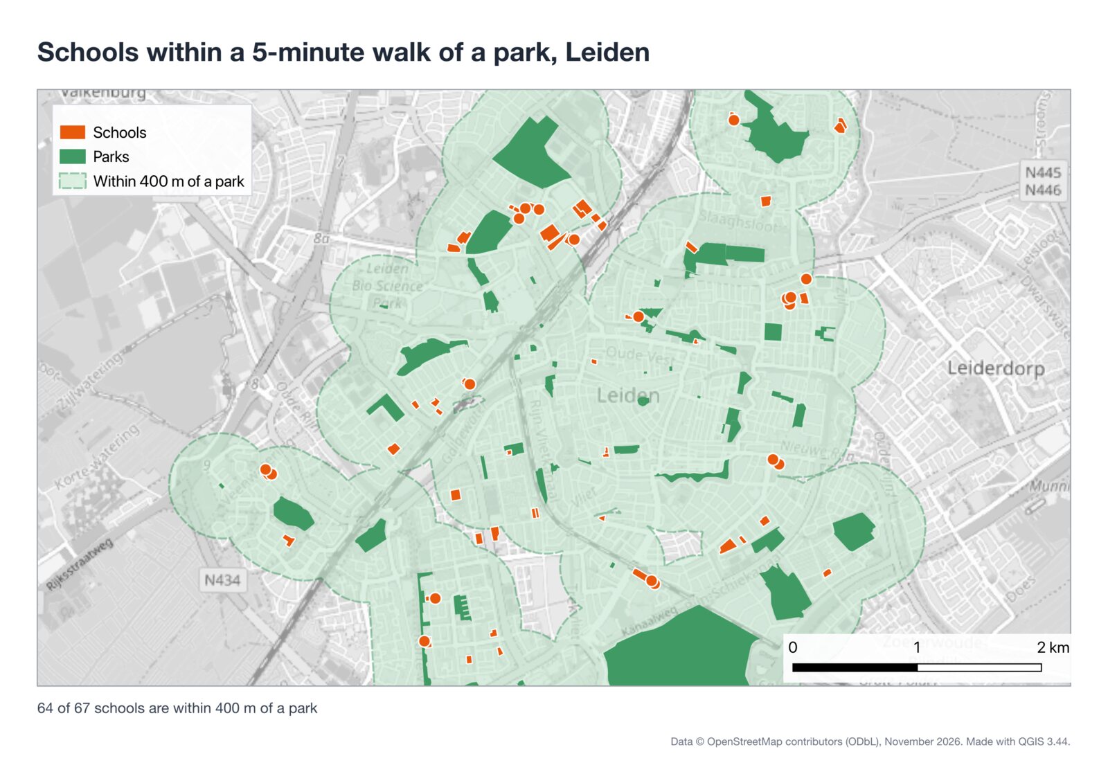
The map answers a question a city planner could ask: how many schools in Leiden, in the Netherlands, are within a 5-minute walk of a park? I built it on 12 November 2026 in QGIS 3.44.15 with free OpenStreetMap data. The answer was 64 of 67.
7steps
From an empty window to a PNG and a PDF
30min
Time to plan for a first session
64/67
Leiden schools within 400 m of a park
51s
The same question asked to AI Agent
What you need before you start
- QGIS, which is free. If it is not on your computer yet, follow how to download and install QGIS, then come back. Any 3.x version works for this tutorial. I used 3.44.15, the long-term release.
- An internet connection, for the basemap and the data.
- No data files. Everything comes from OpenStreetMap during the tutorial.
You can follow along with your own city. Swap "Leiden" for its name in step 3 and pick the right coordinate system in the same step.
Step 1: Learn the 6 parts of the QGIS window (2 minutes)
QGIS looks crowded the first time. Six parts do almost all the work, and you can ignore the rest today.
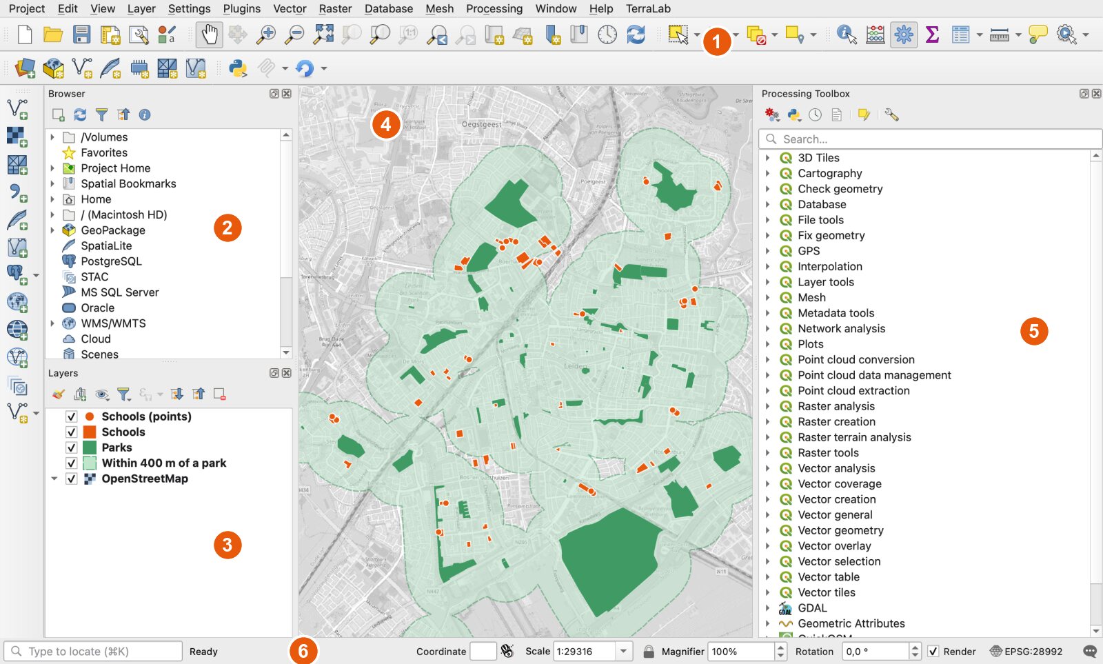
- Menus and toolbars. Every tool lives in a menu. The toolbars are shortcuts to the same tools: the hand pans the map, the magnifiers zoom.
- Browser panel. A file explorer for map data: your folders, plus online sources such as XYZ Tiles.
- Layers panel. The list of what is on your map. The top layer is drawn last, so it covers the ones below. The checkbox shows or hides a layer.
- Map canvas. The map itself. Scroll to zoom, hold the space bar and move the mouse to pan.
- Processing Toolbox. A search box over hundreds of analysis tools. Open it with
Processing > Toolboxif you do not see it. - Status bar. The coordinates under your mouse, the map scale and, at the right end, the coordinate system of the project (for example
EPSG:28992).
If a panel is missing, right-click an empty part of a toolbar and tick its name, or use View > Panels.
Step 2: Add a basemap (3 minutes)
A basemap is a background map that shows you where you are. QGIS ships with one: OpenStreetMap.
Open XYZ Tiles in the Browser
In the Browser panel, scroll down to XYZ Tiles and click the small arrow to open it.
Double-click OpenStreetMap
The world map appears in the canvas and a layer named OpenStreetMap appears in the Layers panel.
Zoom to your city
Scroll in on the Netherlands until Leiden fills the canvas, or click in the locator bar at the bottom left, type
>Leidenand pick the result.
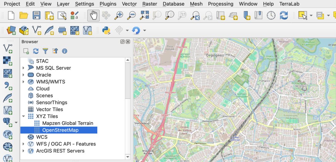
A basemap is a picture. You cannot count its parks or measure its schools. For that you need data, which is the next step. More backgrounds, including aerial imagery, are in how to add a basemap in QGIS.
Now save the project with Project > Save (Ctrl+S, or Cmd+S on a Mac). QGIS writes a .qgz file that remembers your layers and their styles.
Step 3: Load real data from OpenStreetMap (6 minutes)
Map data comes in layers. A vector layer holds shapes (points, lines or polygons), and each shape has a row of attributes such as a name. We need two layers: parks and schools.
The fastest free source is OpenStreetMap, through the QuickOSM plugin. A plugin is an add-on you install from inside QGIS.
Install QuickOSM
Open
Plugins > Manage and Install Plugins, search for QuickOSM and click Install Plugin. It takes a few seconds.Ask for the parks
Open
Vector > QuickOSM > QuickOSMand stay on the Quick query tab. Typeleisureas the key,parkas the value, keep In and typeLeiden. Click Run query.Ask for the schools
Change the key to
amenityand the value toschool, then click Run query again. Close the dialog.
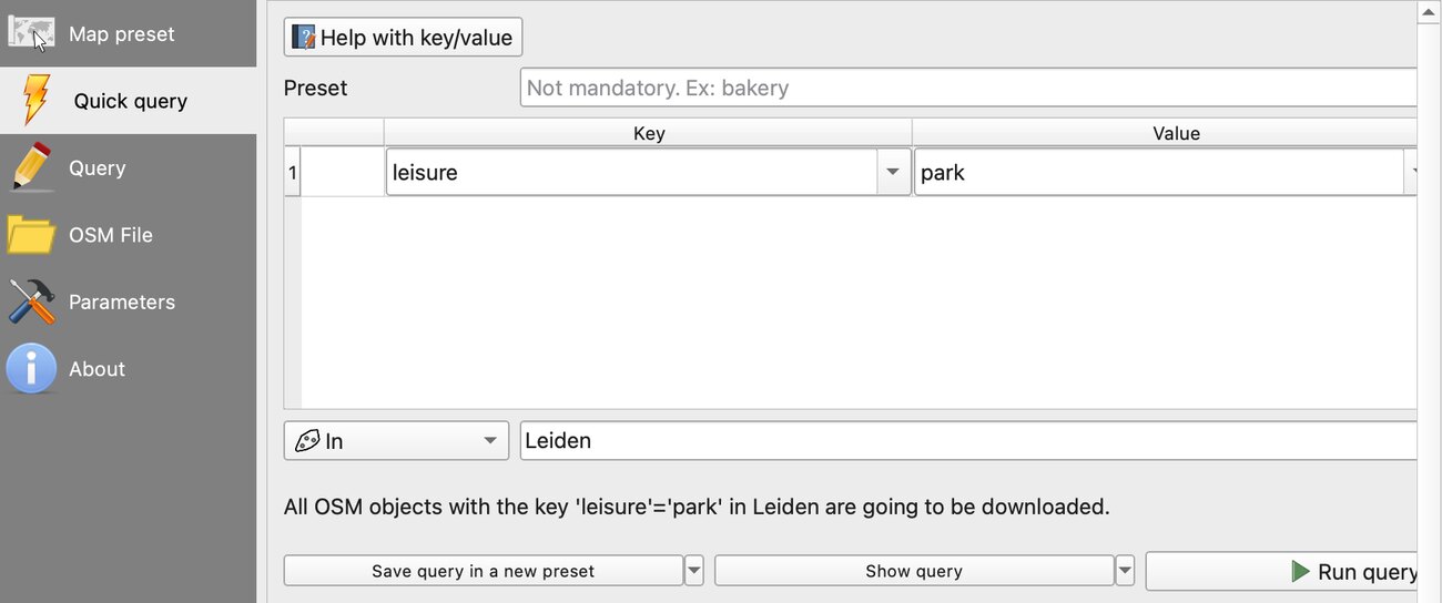
On my run, the parks query took 40.0 seconds and the schools query 27.6 seconds. My very first attempt failed with "Bad Gateway": the public OpenStreetMap server was busy. Running the query again a minute later worked. If it keeps failing, pick another server in the Parameters tab of QuickOSM.
QuickOSM returns one layer per shape type. For Leiden I got:
| Query | Polygons | Points |
|---|---|---|
leisure=park | 56 parks | 10 (ignored here) |
amenity=school | 48 schools drawn as grounds | 19 schools drawn as a single point |
Keep the park polygons and both school layers. Remove the park points: right-click the layer, then Remove Layer.
Save the layers in metres
This is the step beginners skip, and it breaks the analysis later. OpenStreetMap data arrives in latitude and longitude (EPSG:4326), where distances are in degrees. A 400 m buffer needs a coordinate system in metres. If the term is new, what is a CRS explains it in plain words.
The new layers are also temporary: they vanish when you close QGIS. One export fixes both problems.
Export each layer
Right-click the parks layer, then
Export > Save Features As.Choose GeoPackage and a metric CRS
Format: GeoPackage. File name:
leiden.gpkg. Layer name:parks. CRS:EPSG:28992(Amersfoort / RD New, the Dutch national grid). Click OK.Repeat for the schools
Export both school layers into the same
leiden.gpkgfile, with the layer namesschoolsandschool_points. Then remove the three temporary layers.
For another country, type its name in the CRS search box and pick the national grid, or the UTM zone of your city. Then set the project to the same system: click the EPSG code in the status bar and choose it.
Step 4: Style the layers (5 minutes)
QGIS gives each new layer a random colour. Give the map a meaning: green for parks, one strong colour for schools.
Open the Layer Styling panel
Press
F7, or useView > Panels > Layer Styling. Click the Parks layer in the Layers panel.Pick a colour
Click Simple Fill, then the Fill color bar, and choose a green. Set Stroke style to No Line. The map updates as you click.
Style the schools
Select each school layer and choose an orange. Drag the school layers above the parks in the Layers panel so they are drawn on top.
Calm the basemap down
Select OpenStreetMap. In Layer Styling, set Grayscale to By lightness and the opacity to 75%. Your own layers now stand out.
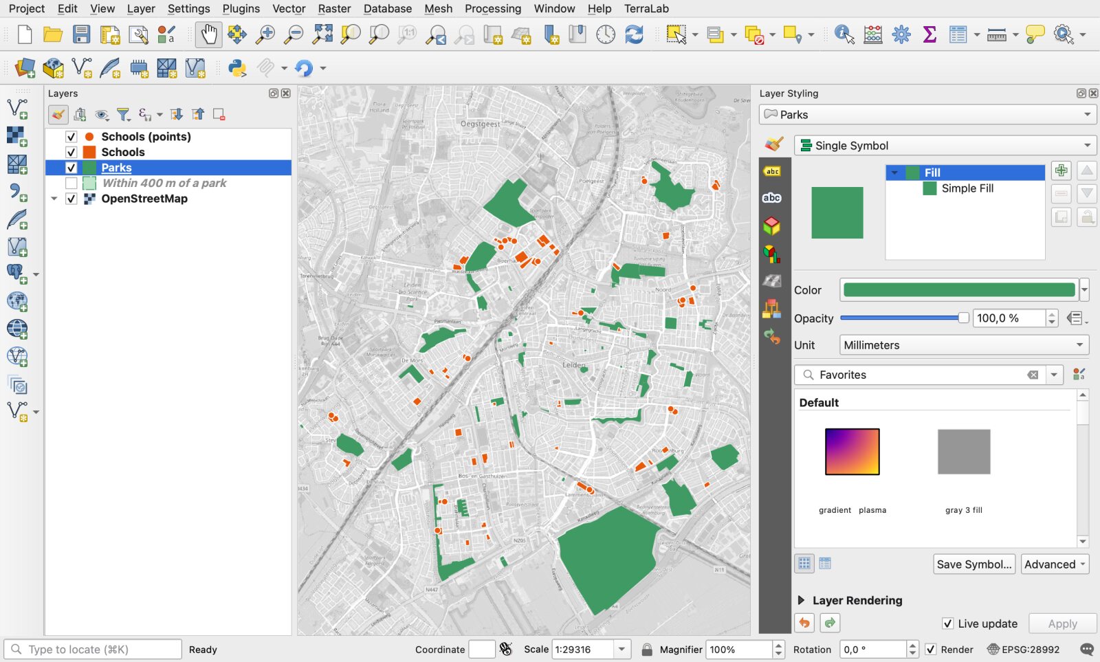
Double-click a layer name to rename it. Those names become the legend in step 7, so write them for a reader: "Parks", "Schools".
Step 5: Read the attribute table (3 minutes)
Every shape carries data. Right-click the Parks layer and choose Open Attribute Table, or press F6.
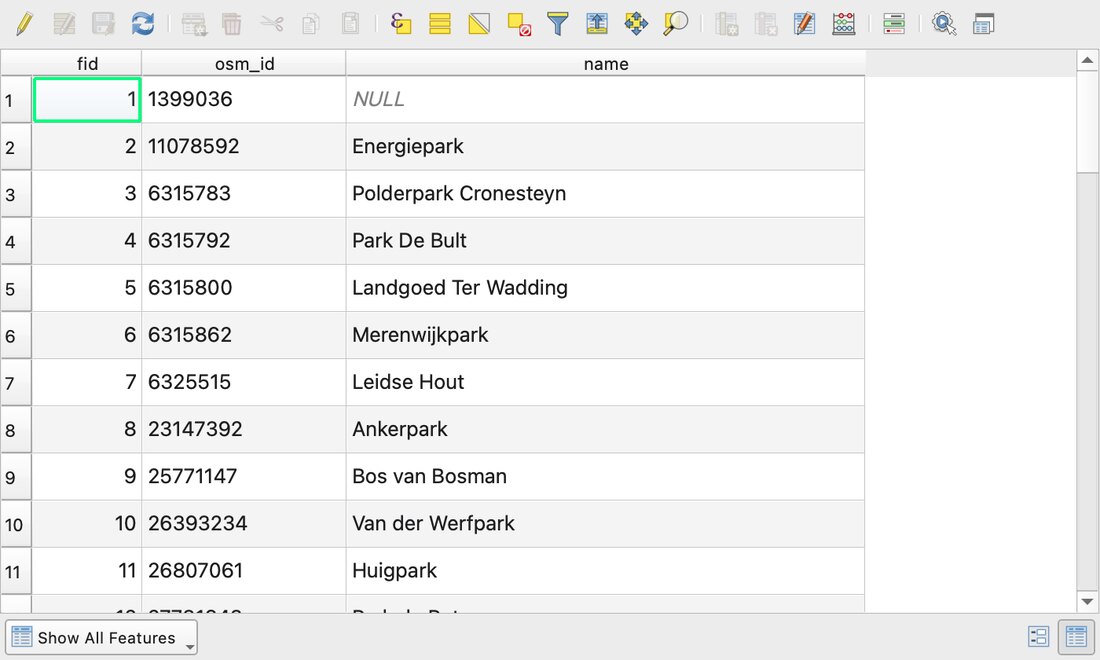
Three things to try:
- Sort. Click a column header.
- Find a park on the map. Click a row number, then the Zoom map to selected rows button in the table toolbar. The park turns yellow on the map.
- Check the gaps. In Leiden, 40 of the 56 parks have a name. Open data is never complete, and the table is where you see it.
To calculate new columns, such as the area of each park, use the QGIS field calculator.
Step 6: Run one analysis: a 400 m buffer (4 minutes)
A common planning rule of thumb counts 400 m as a 5-minute walk. A buffer draws that zone around every park.
Open Buffer
Vector > Geoprocessing Tools > Buffer. You can also type "buffer" in the Processing Toolbox.Set the distance
Input layer: Parks. Distance:
400meters. Tick Dissolve result so the circles merge into one zone. Click Run.Select the schools inside
Vector > Research Tools > Select by Location. Select features from Schools that intersect the Buffered layer. Run it again for the school points.
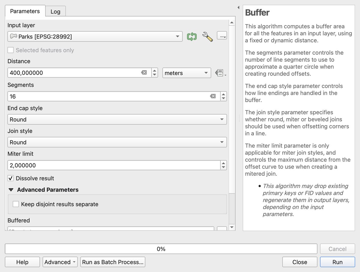
The buffer ran in 0.1 second on 56 parks. If the unit next to the distance says degrees, go back to the export in step 3.
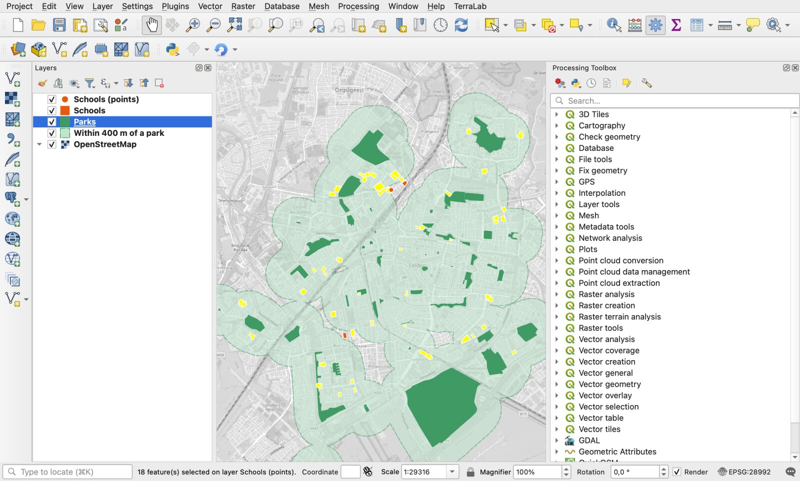
The counts for Leiden: 46 of 48 school grounds and 18 of 19 school points touch the zone. That is 64 of 67 schools within 400 m of a park, and 3 that are not.
Read that number with its limits. The 400 m is a straight line, not a route along streets, and a school drawn twice in OpenStreetMap counts twice. To attach park attributes to each school, the next tool to learn is the spatial join.
Step 7: Build the layout and export the map (7 minutes)
The canvas is your workbench. The print layout is the page you hand to someone: title, legend, scale bar, source.
Create a layout
Project > New Print Layout, give it a name and click OK. A blank A4 page opens in a new window.Add the map
Add Item > Add Map, then drag a rectangle over the page. To reframe it, use the Move item content tool and the mouse wheel.Add a title, a legend and a scale bar
Add Item > Add Labelfor the title and the source line,Add Legend, thenAdd Scale Bar. Click any item to edit it in the Item Properties tab.Clean the legend
In the legend properties, untick Auto update, then remove OpenStreetMap from the list with the minus button.
Export
Layout > Export as Imagefor a PNG,Layout > Export as PDFfor a PDF.
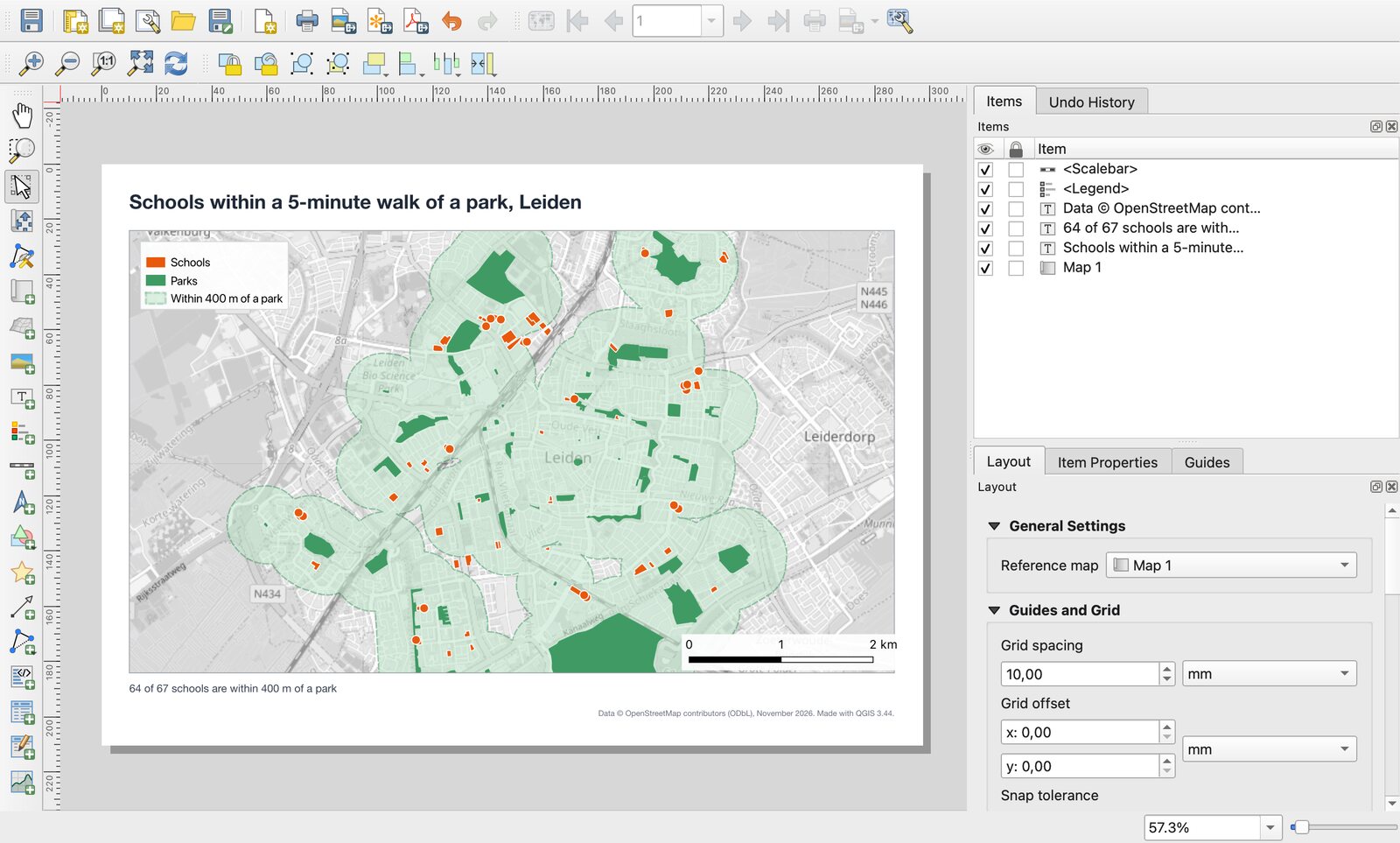
My exports took 2.4 seconds for the PNG at 200 dpi (2.0 MB) and 1.9 seconds for the PDF (1.6 MB). Always credit the data on the page: for OpenStreetMap the line is "© OpenStreetMap contributors".
For better maps (labels, a north arrow, classes of colour), continue with how to make a map in QGIS.
The same map from one sentence
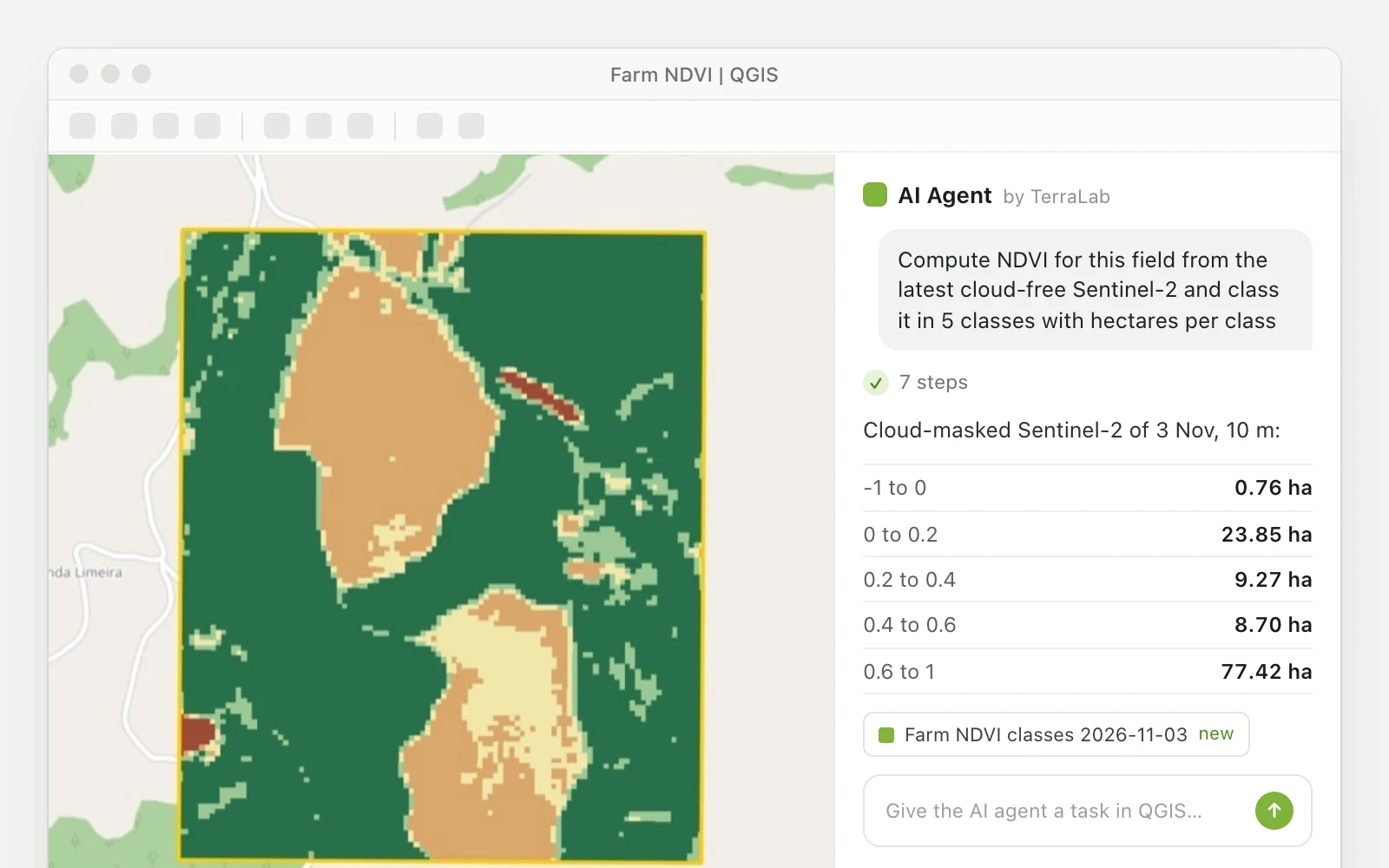
QGIS also takes plugins that do the clicking for you. I work on one of them, AI Agent: a panel inside QGIS where you write what you want and it runs the QGIS tools itself.
I opened a new project with only the OpenStreetMap basemap and sent this sentence:
Map the schools in Leiden, Netherlands that are within a 5-minute walk (400 m) of a park, using OpenStreetMap data. Tell me how many schools are inside and how many are not.
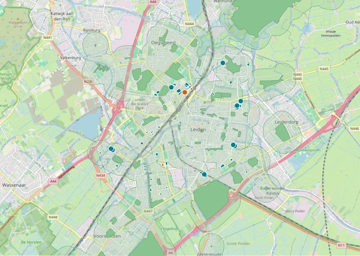
The run took 51 seconds. It downloaded both datasets, reprojected them to the Dutch grid on its own, buffered the parks, coloured the schools by result and answered: 58 of 61 school features within 400 m, 3 beyond. It also wrote the two limits I gave above without being asked: straight-line distance, and features that are not always unique schools.
Why 58 of 61 and not 64 of 67? The two routes did not use the same data. I asked QuickOSM for objects inside the municipality of Leiden. AI Agent downloaded the area around the city, so it found 88 park polygons, some in neighbouring towns, and 13 school points where I had 19. Both counts are correct for their own definition. A number on a map depends on where you drew the boundary, and writing that boundary down is part of the work.
Limits of each route. By hand, you learn where every tool lives and you control each choice, and the first time takes half an hour. With AI Agent, the first result comes in under a minute, but you must read what it did, and it gives you layers on the canvas, not a finished print layout: step 7 is still yours, or a second request. The Free plan covers 5 tasks a month.
My advice for a beginner: do the seven steps by hand once. After that, use the agent for the routine parts and keep your attention for the question and the checks. The AI Agent guide shows a full project done that way.
Five beginner mistakes this tutorial avoids
- Buffering in degrees. Save layers in a metric coordinate system before any distance tool (step 3).
- Losing temporary layers. A layer with a small chip icon next to its name lives in memory only. Export it to a GeoPackage.
- Treating the basemap as data. You cannot select or count what is in a basemap.
- Moving the data files. The project file stores paths, not the data. Keep the
.qgzand the.gpkgin one folder and move them together. - Forgetting the source. A map without a data credit cannot be published.
What to learn next
- More data: download OpenStreetMap data in QGIS, with larger areas and other methods.
- Better backgrounds: add a basemap, including aerial imagery.
- Old maps and scans: georeference an image so it lines up with your layers.
- Combine layers: the spatial join and the field calculator.
- Cartography: make a map in QGIS, step by step.
- Extend QGIS: the best QGIS plugins, and AI Agent when you would rather describe the task than look for the tool.
How I measured this. Everything ran on 12 November 2026 on an Apple Silicon Mac (macOS 27.0.1) in QGIS 3.44.15 with QuickOSM 2.5.3 and AI Agent 1.9.5, signed in to a Pro test account with its default settings. The seconds are measured: the two downloads, the buffer, the two exports and the AI Agent run. The minutes in the step titles are a budget for a first session, not a stopwatch reading. I prepared the session with scripts, so I did not time my own clicks. OpenStreetMap changes every day: your counts will differ a little.
Frequently asked questions
Start with one small project instead of a tour of every menu. Add the OpenStreetMap basemap from XYZ Tiles in the Browser panel, load one or two layers, style them in the Layer Styling panel (F7), run one tool such as Buffer, and export a map from a print layout. Those seven steps, shown above on schools and parks in Leiden, use the six parts of the window you will need in every later project.
The basics are not. A first map takes about 30 minutes with a guide. What takes longer is the knowledge around the software: coordinate systems, data formats and choosing the right analysis tool among hundreds. Learn those one project at a time. The official QGIS Training Manual covers them in depth for free.
Yes. QGIS is free and open source under the GNU General Public License. There is no paid edition, no trial period and no feature locked behind a licence, for personal or commercial work. Some plugins made by companies have paid plans, but QGIS itself costs nothing. See what is QGIS for more.
Printed and web-ready maps, and the analysis behind them: distance zones, counts by area, elevation and slope maps, routes, satellite image indices such as NDVI, and georeferenced old plans. It reads and writes most formats, including Shapefile, GeoPackage, GeoJSON, KML, CSV and GeoTIFF.
Right-click a layer in the Layers panel, choose Export > Save Features As, set the format to GeoPackage, pick a file name and a layer name, and click OK. To add more layers to the same file, export them to the same file name with a different layer name. Step 3 above does this for parks and schools.
Yes. QGIS is free, open data such as OpenStreetMap is free, and the official Training Manual and many written tutorials cost nothing. Pick a question about a place you know, build the map, then repeat with a harder question. An assistant such as AI Agent can also explain each tool it runs, which helps when you do not know the name of what you need.
Open Settings > Options > General, tick Override system locale, choose the language in User interface translation, and restart QGIS. On a Mac, the Options entry is under the QGIS menu, named Preferences.
Read nextHow to Make a Map in QGIS: Step by Step, Then With AI
Do it in QGIS by asking for it
AI Agent carries out the task you describe, in your own QGIS project. Free, no card.